Reducing the complexity of calculations in operations with vectors and matrices

Introduction

Due to the fact that when solving optimization problems, differential games, and in 2D and 3D calculations, or rather when writing software that performs calculations to solve them, some of the most frequently performed operations are vector-matrix transformations of the type $$$aX + bY$ where $$$a, b$ - scalar values $$$X, Y \ in R ^ n$ - vector or matrix of dimension $$$R ^ {n \ times m}$ .

Actually these are:

( source ).

So, in order not to delve into the theory of optimization for examples, it suffices to recall the fourth order Runge-Kutta numerical integration formula:

$$

$$Y_ {n + 1} = Y_n + \ frac {h} {6} (k_1 + 2 k_2 + 2 k_3 + k_4),$$

Where $$$Y_i$ - the next value of the integrable function $$$f (t, Y)$$$$h$ - method step, and $$$k_i$ , $$$i = 1..4$ - values ​​of the integrable function at some intermediate points - in the general case of vectors.

As you can see, the main mass of mathematical operations for both vectors and matrices are:

• addition and subtraction are faster;
• multiplication and division are slower.

The complexity of the calculations is well written in the corresponding MIPT course .

In addition, quite significant costs in the implementation of vector calculations fall on memory management operations - the creation and destruction of arrays of matrices and vectors.

Accordingly, it makes sense to do a decrease in the number of operations that introduce the greatest complexity - multiplication (mathematics) and memory management operations (algorithmic).

Reduced computational complexity

Arbitrary vector $$$x \ in R ^ n$ present in the form $$$x = aX$ where
$$$a \ in R ^ 1$ , $$$X \ in R ^ n$ , we denote as $$$[a, X]$ . The operation of bringing such a vector is called the calculation $$$[a, X] = x \ in R ^ n$ , Is the inverse operation whose computational complexity is $$$n$ multiplication operations.

Accordingly, by saving we mean the saving of multiplication operations.

What can you save on operations with vectors:

1. Multiplication by a constant $$$b [a, X] = [ab, X]$ - saved $$$n-1$ multiplication operation.
2. Addition $$$k$ directed vectors $$$\ sum \ limits_ {i = 1} ^ {k} [a_i, X] = \ left [\ sum \ limits_ {i = 1} ^ {k} a_i, X \ right]$
   
   • delayed calculation $$$n$ multiplications;
   • saved $$$(k-2) n$ multiplications.
3. Addition of non-aligned vectors $$$[a, X] + [b, Y] = [a, X + b / a \ Y]$ - calculation is postponed $$$n-1$ multiplication operation, with $$$a \ ne 0$ .
4. Matrix vector multiplication: $$$A [a, x] = [a, Ax]$ where $$$A \ in R ^ {m \ times n}$ - which allows you to delay the calculation $$$m$ multiplication operations.
5. Dot product of vectors $$$([a, X], [b, Y]) = ab (X, Y)$ - saved $$$n-1$ an operation of real multiplication.

Similarly, if we represent the matrix in the form $$$Y = a \ bar Y$ where
$$$a \ in R ^ 1$ , but $$$\ bar Y, Y \ in R ^ {n \ times m}$ , we denote as $$$[a, \ bar Y]$ . Accordingly, the cast operation - calculation $$$[a, \ bar Y] = Y \ in R ^ {n \ times m}$ , Is the inverse operation whose computational complexity is $$$n \ cdot m$ multiplication operations.

The possibilities of saving (1–4) are similar, with the only difference being that the operation of the scalar product (5) is absent, and for the remaining operations the possibility of saving multiplication becomes greater in $$$m$ times, which is quite nice, especially when it is necessary to store arrays of vectors in a matrix representation for performing various mass operations on them.

It is clear that the above methods of saving are not free in the sense of the need to have additional memory for storing coefficients, and overhead costs associated with monitoring the state of the calculated objects.

In addition to purely mathematical optimizations, this approach is fully applicable to calculations on grids, for example, if the value of a grid function represented by a vector must first be multiplied by some constant, and then its maximum can be found using the gradient method (without going through all the values).

Reduced algorithmic complexity

As can be seen from the preceding arguments, real savings arise for:

• multiplying the vector / matrix by the number and scalar products of vectors;
• operations on vectors and matrices that differ only by coefficients.

Accordingly, in order to ensure the optimization of scalar calculations, it is necessary to construct a data structure of the following form:

class Vector { public: sVec *v; //   double upd; //. a bool updated; // ,  a==1 //.... }; 

Perhaps not the most obvious here - the assignment of the variable is updated , in view of the fact that if upd = 1 , then it seems like additional checks are redundant. But if we recall that the consistent division and multiplication of the following form:

 a_ /= b_; a_ *= b_; 

It is not obliged to maintain the value of a_ due to rounding, it is clear that this insurance is not superfluous.

Further, if you pay attention to the fact that if the vectors $$$[a, X]$ and $$$[b, x]$ myself $$$X$ it’s the same, it makes no sense to store it twice, but it’s enough to create a single object of the base vector class $$$X$ and refer to it in the calculations, i.e.

 class sVec { public: unsigned long size; double *v;//   long linkCount;//  //.. };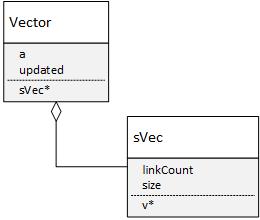 

The dynamic array here is necessary to work out the tendency of the vectors to change the dimension when multiplying by the matrix, the approach associated with reference to the links is in order to remove the logic associated with creating and tracking duplicates of objects using the overloaded operators for vector and matrix operations in C ++.

Features of the implementation

For an example (which can be taken on github), we consider fairly simple calculations related to vector-matrix arithmetic in terms of economy of multiplication operations. So: first create the necessary objects:

  Vector X(2), Y(2), Z(2); //   R^2 double a = 2.0; // .      

and initialize them as a unit vector for X = [1,1] and zero for Y = [0,0]

  X.one(); //  [1,1] Y.zero();//    [0,0] cout<<" X: "<<X<<"   X: "<<Xv->linkCount<<"  : "<<Xv<<endl; cout<<" Y: "<<Y<<"   Y: "<<Yv->linkCount<<"  : "<<Yv<<endl; 

We get that the internal vectors indicate the expansion of the arrays and both reference counters are equal to one.

  X: [1,1];   X: 1  : 448c910  Y: [0,0];   Y: 1  : 448c940 

Further we equate vectors:

  Y=X;//   X  Y cout<<" X: "<<X<<"   X: "<<Xv->linkCount<<"  : "<<Xv<<endl; cout<<" Y: "<<Y<<"   Y: "<<Yv->linkCount<<"  : "<<Yv<<endl; 

and we see that now both vectors point to the same address, and the link count has increased by 1:

  X: [1,1];   X: 2  : 448c910  Y: [1,1];   Y: 2  : 448c910 

Then multiply the vector X by 2

  X*=a; //    2.0 cout<<" X: "<<X<<"   X: "<<Xv->linkCount<<"  : "<<Xv<<" . a  X: "<<X.upd<<endl; cout<<" Y: "<<Y<<"   Y: "<<Yv->linkCount<<"  : "<<Yv<<" . a  Y: "<<Y.upd<<endl; 

and we get that, despite the fact that both vectors, as before, point to the same address, and the reference counter, as before, 2, y. X stored coefficient is 2, and Y is respectively equal to 1:

  X: [2,2];   X: 2  : 448c910 . a  X: 2  Y: [1,1];   Y: 1  : 448c910 . a  Y: 1 

And at the end, folding X + Y

  Z= X+Y; cout<<" Z: "<<Z<<"   Z: "<<Zv->linkCount<<"  : "<<Zv<<" . a  Z: "<<Z.upd<<endl; 

we get Z = [3,3] :

  Z: [3,3];   Z: 1  : 448c988 . a  Z: 1 

For matrices, all calculations are similar:

  Matrix X_(2), Y_(2), Z_(2); // 3    2x2 cout<<" X: "<<endl<<X_<<"   X: "<<X_.v->linkCount<<"  : "<<X_.v<<endl; cout<<" Y: "<<endl<<Y_<<"   Y: "<<Y_.v->linkCount<<"  : "<<Y_.v<<endl; Y_=X_;//   X_  Y_ cout<<" X: "<<endl<<X_<<"   X: "<<X_.v->linkCount<<"  : "<<X_.v<<endl; cout<<" Y: "<<endl<<Y_<<"   Y: "<<Y_.v->linkCount<<"  : "<<Y_.v<<endl; X_*=a; //    2.0 cout<<" X: "<<endl<<X_<<"   X: "<<X_.v->linkCount<<"  : "<<X_.v<<" . a  X: "<<X_.upd<<endl; Z_= X_+Y_; cout<<" Z: "<<endl<<Z_<<"   Z: "<<Z_.v->linkCount<<"  : "<<Z_.v<<" . a  Z: "<<Z_.upd<<endl; 

The output is also similar:

  X: [1,0] [0,1];   X: 1  : 44854a0  Y: [1,0] [0,1];   Y: 1  : 44854c0  X: [1,0] [0,1];   X: 2  : 44854a0  Y: [1,0] [0,1];   Y: 2  : 44854a0  X: [2,0] [0,2];   X: 2  : 44854a0 . a  X: 2  Z: [3,0] [0,3];   Z: 1  : 4485500 . a  Z: 1 

The library is available on GitHub .

Use, criticize.