Descriptor graphics in MATLAB: the second horizontal axis
When studying descriptor graphics in MATLAB, there was a shortage of “user friendly” functionality, namely the absence of a standard command that allows you to add an additional horizontal axis.
Adding an additional vertical axis, the plotyy command also provides for help to it, in the topics section, there is an example of adding an additional x axis, however this example, like the command itself, is not without flaws, which the developer himself kindly informs us with the phrase:
Perhaps we omit the analysis of the shortcomings of the team itself, but it is worth mentioning the shortcomings of the example specified by the developers:
To solve the above problems, we will write our code:
')
Let's take a closer look at some code elements:
Using the command below, we obtain the position of the axes in the form of a numeric array.
The array ax is represented as [abcd], where a and b are the position of the lower left corner of the graph, horizontally and vertically, respectively. That is, the coordinates of the origin; c is the length of the horizontal axis, d is the length of the vertical axis.
Introducing offsets, no golden section was calculated, everything was “by eye”:
So, ax (2) + (ax (2) / 2) - shifts the beginning of the standard axis vertically to half of the current one, i.e. up from the initial position, which is necessary for readability of the numbered scale marks. The offset ax (4) -ax (4) / 10 sets the size of the first axes along the vertical, i.e. reduces by one tenth of the current value, it is necessary for readability of the schedule signature, recall the title . If you set d = 0, then the vertical axis will simply not be visible, which we will use in the case of:
The following code allows you to set the position of the labels of the horizontal axes:
The BX array, as well as BY, is represented as [xy], where x is the horizontal position of the signature, y is the vertical position of the signature.
Below I will leave a couple of useful links.
command description axes ;
settings command axes ;
plotyy command ;
method of introducing an additional horizontal axis from the developers .
Adding an additional vertical axis, the plotyy command also provides for help to it, in the topics section, there is an example of adding an additional x axis, however this example, like the command itself, is not without flaws, which the developer himself kindly informs us with the phrase:
plotyy is not recommended
Perhaps we omit the analysis of the shortcomings of the team itself, but it is worth mentioning the shortcomings of the example specified by the developers:
- Firstly, we are offered to locate an additional axis in the moveometonic area itself - at the top of the graph. Eyes scatter when trying to analyze such a picture ...
- Secondly, it may not be clear how to sign such an axis even to an advanced matlab user;
- Third, why do we need another y axis?
Help code
figure x1 = 0:0.1:40; y1 = 4.*cos(x1)./(x1+2); line(x1,y1,'Color','r') title(' ') % ax1 = gca; % current axes ax1.XColor = 'r'; ax1.YColor = 'r'; ax1_pos = ax1.Position; % position of first axes ax2 = axes('Position',ax1_pos,... 'XAxisLocation','top',... 'YAxisLocation','right',... 'Color','none'); x2 = 1:0.2:20; y2 = x2.^2./x2.^3; line(x2,y2,'Parent',ax2,'Color','k') xlabel('f,') % I visualize an example of help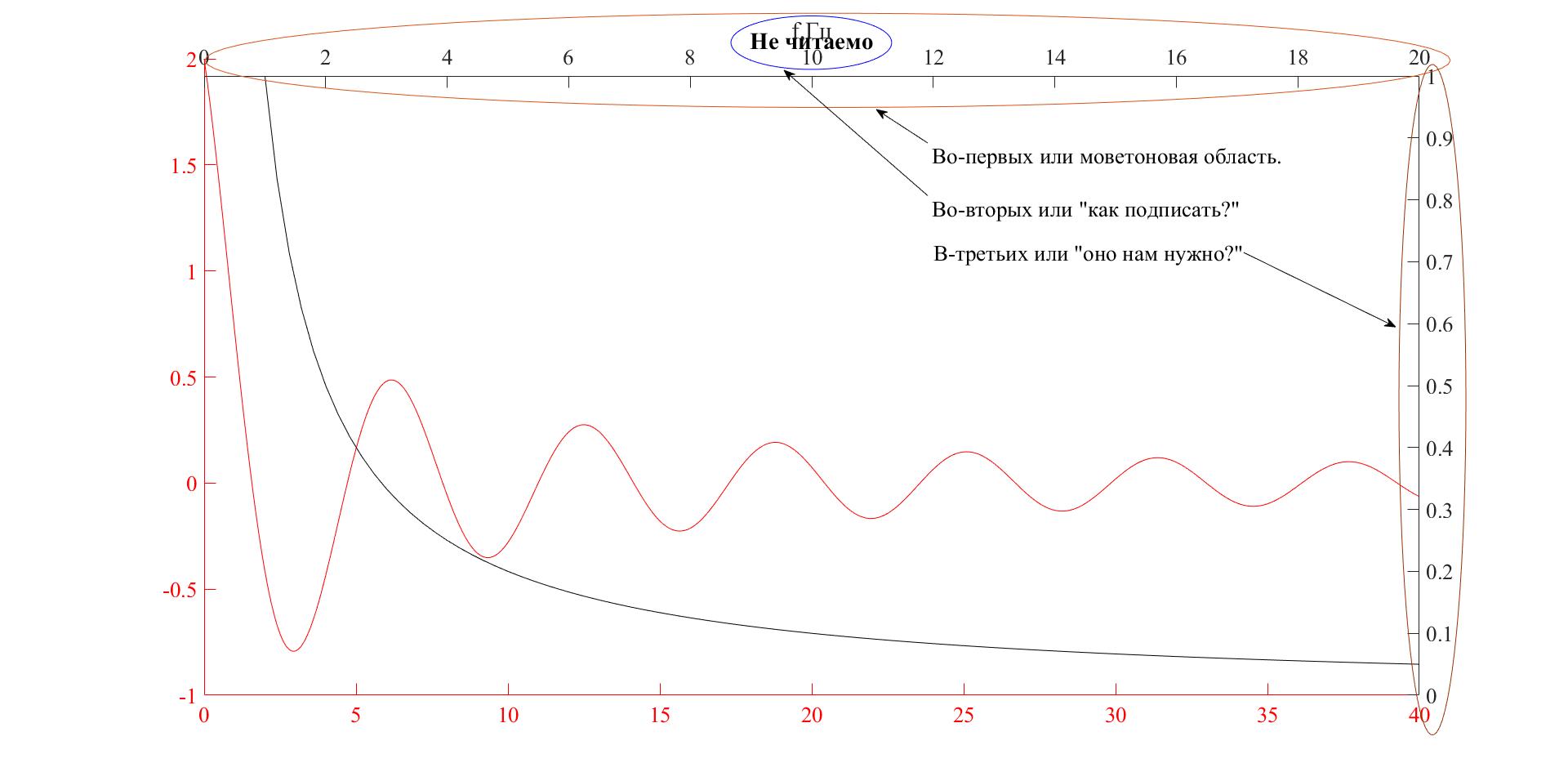
To solve the above problems, we will write our code:
')
Problem solving
clc clear all close all %% , U=[5.5 5.5 5.5 5.2 5.1 5 5 4.8 4.8]; % F=[30 40 50 10000 12000 14000 16000 18000 20000]; % [xi,ni]=find(F==50); K=U/U(ni); % %% figure %% , set(0,'DefaultAxesFontSize',20,'DefaultAxesFontName','Times New Roman'); set(0,'DefaultTextFontSize',20,'DefaultTextFontName','Times New Roman'); %% , ax=get(axes,'Position'); % a=gca; % set(a,'Position',[ax(1) ax(2)+(ax(2)/2) ax(3) ax(4)-ax(4)/10]) % plot(a,log(F),K,'-o'); % xlim(a,[min(log(F)) max(log(F))]) % grid on % BX=get(gca,'XTick'); % x BY=get(gca,'YTick'); % y %% xlabel('','Position',[BX(size(BX,2))+1.1 BY(1)+(BY(1)/100)]) ylabel('K(f)') %% F1=num2str(F,'%0.0i\n'); % ax2=[ax(1) ax(2)-(ax(2)/4) ax(3) 0]; % b=axes('Position',ax2); % xlabel('f, ', 'Position',[BX(size(BX,2))+1.1 BY(1)+(BY(1)/100)]) % xlim(b,[min(log(F)) max(log(F))]) % , xticks(b,log(F)) % xticklabels(b,F1) % xtickangle(90) % , Let's take a closer look at some code elements:
Using the command below, we obtain the position of the axes in the form of a numeric array.
ax=get(axes,'Position'); The array ax is represented as [abcd], where a and b are the position of the lower left corner of the graph, horizontally and vertically, respectively. That is, the coordinates of the origin; c is the length of the horizontal axis, d is the length of the vertical axis.
Introducing offsets, no golden section was calculated, everything was “by eye”:
set(a,'Position',[ax(1) ax(2)+(ax(2)/2) ax(3) ax(4)-ax(4)/10]) So, ax (2) + (ax (2) / 2) - shifts the beginning of the standard axis vertically to half of the current one, i.e. up from the initial position, which is necessary for readability of the numbered scale marks. The offset ax (4) -ax (4) / 10 sets the size of the first axes along the vertical, i.e. reduces by one tenth of the current value, it is necessary for readability of the schedule signature, recall the title . If you set d = 0, then the vertical axis will simply not be visible, which we will use in the case of:
ax2=[ax(1) ax(2)-(ax(2)/4) ax(3) 0]; The following code allows you to set the position of the labels of the horizontal axes:
BX=get(gca,'XTick'); BY=get(gca,'YTick'); xlabel('','Position',[BX(size(BX,2))+1.1 BY(1)+(BY(1)/100)]) xlabel('f, ', 'Position',[BX(size(BX,2))+1.1 BY(1)+(BY(1)/100)]) The BX array, as well as BY, is represented as [xy], where x is the horizontal position of the signature, y is the vertical position of the signature.
As a result, we can see such beauty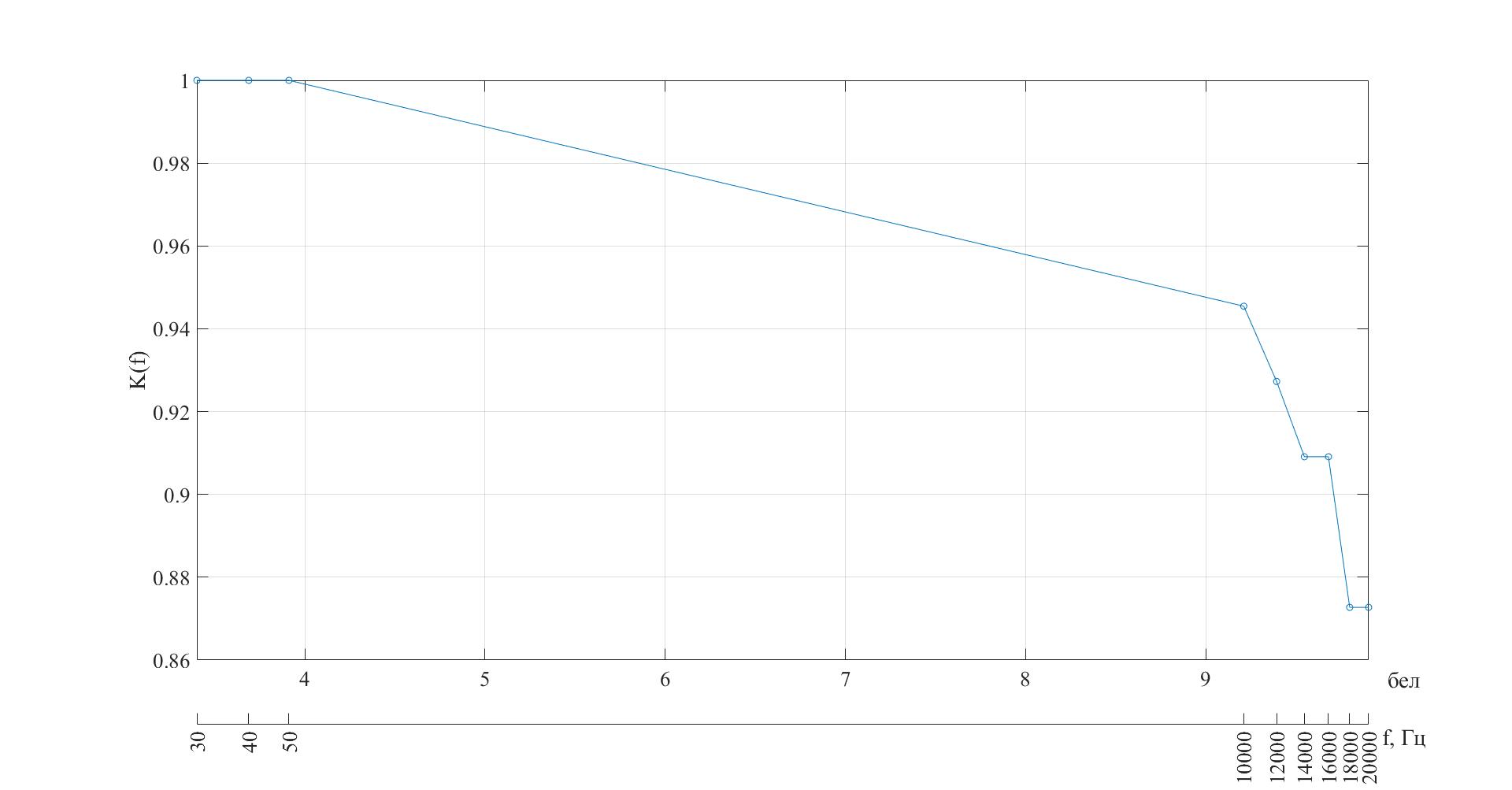
Below I will leave a couple of useful links.
command description axes ;
settings command axes ;
plotyy command ;
method of introducing an additional horizontal axis from the developers .
Source: https://habr.com/ru/post/350836/
All Articles