Suspended fuel tanks for aircraft

Introduction
Often, to ensure long-range, additional tanks are suspended from the outside of the aircraft. Suspended tanks can be discharged and not discharged.
Suspended outboard tanks, after the use of fuel from them, are dumped in the same way as aerial bombs from the locks of bomb racks on which they are hung.
')
The power supply from the outboard tanks is carried out by switching on the pipelines from these tanks into the general system for supplying the engine with fuel through a stop or multi-way valve.
An interesting fact is that in the Vietnamese jungle after the war they began to find a lot of fuel tanks dropped by American planes.
Peasants saw tanks along and make two boats. Such a boat does not rust, weighs little, and thanks to the aerodynamic shape on it is very easy to row.

It would be nice to have such a boat, but at the same time, I don’t really want the aircraft with outboard tanks to fly over us.
Aerodynamic resistance (AC) of the outboard fuel tank
Depending on the flight mode and the shape of the tank, one or another aerodynamic drag component will prevail. For example, for blunt bodies of revolution moving at high supersonic speeds, the resistance has a wave character.
For well-streamlined bodies moving at low speeds, friction resistance and eddy-loss losses prevail.
The vacuum that occurs on the rear end surface of the streamlined body, also leads to the resultant force directed opposite to the velocity of the body.
Aerodynamic resistance Fa is characterized by a dimensionless aerodynamic drag coefficient Cx:

where ρ is the density of the unperturbed medium, v is the velocity of the body relative to this medium, S is the characteristic area of the body, Cx is the dimensionless coefficient of aerodynamic drag, usually determined experimentally, and for simple forms of rotation and calculation.
The layout of the outboard fuel tank of rotation bodies according to the criterion of the minimum area S and coefficient Cx
We use the data on the calculation of the drag coefficient (Cx) of simple bodies and the comparison of the obtained result with the experiment given in the publication [1]:

For bodies of rotation, located at the ends of the tank with the cylinder between them (to hold the bulk of the fuel),
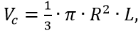 surface area
  You can choose the following layout options:
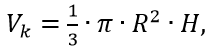
cone (with H = R) –volume
 surface area
cone (at H <> R) –volume
 surface area
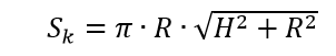
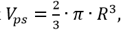
hemisphere –volume
 surface area
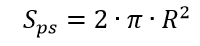


Let us set a tank volume of 3 m3: Vb = Vps + Vc + Vk, Vb = 3, determine the dimensions for the optimal layout from the following listing, when the condition for the minimum Cx (2h = d or H = R) is not met:
# -*- coding: utf8 -*- import numpy as np from scipy.optimize import minimize import matplotlib.pyplot as plt def objective(x):# - x1=x[0]# R x2=x[1]# H , H=R x3=x[2]# L return 2*np.pi*x1**2+2*np.pi*x1*x3+np.pi*x1*((x1**2)+(x2**2))**0.5 def constraint(x): # return (2/3)*np.pi*(x[0]**3)+np.pi*x[2]*(x[0]**2)+(1/3)*x[1]*np.pi*(x[0]**2)-3 x0=[1,1,1]# b=(0.0,1)# bnds=(b,b,b) con={'type': 'ineq','fun':constraint} res = minimize(objective, x0,bounds=bnds,constraints=con) e=round(res['fun'],3) e1=round(res['x'][0],3) e2=round(res['x'][1],3) e3=round(res['x'][2],3) print (" :%s"%e) print (" :%s"%e1) print (" :%s"%e2) print (" :%s"%e3) We get:
Estimated value of the area of the outboard tank: 10.253
Estimated value of hanging tank radius: 0.878
The estimated value of the height of the cone hanging tank: 0.785
The estimated value of the length of the cylinder outboard tank: 0.393
For a given tank volume Vb = 3, we determine the dimensions for the optimal layout from the following listing, when the condition for the minimum Cx (2h = d or H = R) is fulfilled:
# -*- coding: utf8 -*- import numpy as np from scipy.optimize import minimize import matplotlib.pyplot as plt def objective(x):# - x1=x[0] # R , H=R x2=x[1]# L return 2*np.pi*x1**2+2*np.pi*x1*x2+np.pi*x1*(2*(x1**2))**0.5 def constraint(x): # return (2/3)*np.pi*(x[0]**3)+np.pi*x[1]*(x[0]**2)+(1/3)*x[0]*np.pi*(x[0]**2)-3 x0=[1,1]# b=(0.0,1)# bnds=(b,b) con={'type': 'ineq','fun':constraint} res = minimize(objective, x0,bounds=bnds,constraints=con) e=round(res['fun'],3) e1=round(res['x'][0],3) e2=round(res['x'][1],3) print (" :%s"%e) print (" :%s"%e1) print (" :%s"%e1) print (" :%s"%e2) We get:
Estimated value of the hanging tank area: 10.259
Estimated value of hanging tank radius: 0.877
The estimated value of the height of the cone hanging tank: 0.877
The estimated value of the length of the cylinder outboard tank: 0.363
Conclusion:
In comparison with the option when the condition R = H is not met, the total surface area of the tank has hardly changed. This layout is optimal, which is confirmed by practice.
Numerical values are given for example, in each case, you need to consider the design features.
Measurement of fuel level in the outboard fuel tank
The operation of a jet engine depends on the flow rate of the fuel supplied, which is adjusted to the level in the tank. Therefore, the measurement of the fuel level in the tank is an important technological parameter.
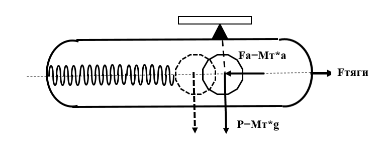
In the non-discharged fuel tank, the fuel level is measured by sensors installed in a straight channel, the upper open end of which is located above the fuel level, which fills the channel due to the charge pressure Po.
The vertical channel and fuel tank are communicating vessels. By lowering the fuel level in the tank, the fuel level decreases in the channel. When the fuel level in the channel reaches the sensor, the sensor is activated. The signal enters the fuel management system.
Thus, the level of fuel in the channel determines the level of fuel in the tank. The problem is that the free surface of the fuel does not match in the channel and the reservoir. An error in measuring the fuel level leads to inefficient fuel consumption.

The fuel level in the tank varies according to the ratio:

where: Ho - the initial level of fuel in the tank; V– fuel feed rate; t is time.
For further analysis of the dependence of the fuel supply rate on time, we use the ratio obtained in the publication [2]:

where: y - coordinates of the free surface of the fuel in the measuring channel; L is the coefficient of friction of the fluid against the walls of the cylindrical measuring channel; R is the radius of the cylindrical measuring channel; g - gravitational acceleration.
The initial conditions for the differential equation (1) are:
y (0) = Ho, dy / dt = 0.
For the numerical solution of the differential equation (1) by means of Python, we introduce the following notation:

The change in the average fuel velocity in the measuring channel.
# -*- coding: utf8 -*- import numpy as np from scipy.integrate import odeint import matplotlib.pyplot as plt R=0.0195 H=8.2 g=9.8 L=4.83*10**-2 V=0.039 def f(y,t): y1,y2=y return [y2,-g+(g*(HV*t)/y1)+((L/(4*R))*y2**2)] t = np.arange(0,200,0.01) y0=[H,0] [y1,y2]=odeint(f,y0,t,full_output=False).T plt.title(" \n ") plt.xlabel("t,s") plt.ylabel("U,m/s ") plt.plot(t,y2) plt.grid(True) plt.show() We get:

Fuel levels in the measuring channel and in the tank.
# -*- coding: utf8 -*- import numpy as np from scipy.integrate import odeint import matplotlib.pyplot as plt R=0.0195 H=8.2 g=9.8 L=4.83*10**-2 V=0.039 def f(y,t): y1,y2=y return [y2,-g+(g*(HV*t)/y1)+((L/(4*R))*y2**2)] t = np.arange(0,10,0.01) y0=[H,0] [y1,y2]=odeint(f,y0,t,full_output=False).T plt.title(' ') plt.ylabel('H,m') plt.ylabel('t,s') plt.plot(t,y1,"b",linewidth=2,label=' ') y=HV*t plt.plot(t,y,"--r",linewidth=2,label=' ') plt.grid(True) plt.legend(loc='best') plt.show() We get:

Error measuring fuel level.
# -*- coding: utf8 -*- import numpy as np from scipy.integrate import odeint import matplotlib.pyplot as plt R=0.0195 H=8.2 g=9.8 L=4.83*10**-2 V=0.039 def f(y,t): y1,y2=y return [y2,-g+(g*(HV*t)/y1)+((L/(4*R))*y2**2)] t = np.arange(0,200,0.01) y0=[H,0] [y1,y2]=odeint(f,y0,t,full_output=False).T plt.title(' ') plt.ylabel('d,m') plt.xlabel('t,s') d=y1-(HV*t) plt.plot(t,d) plt.grid(True) plt.show() We get:
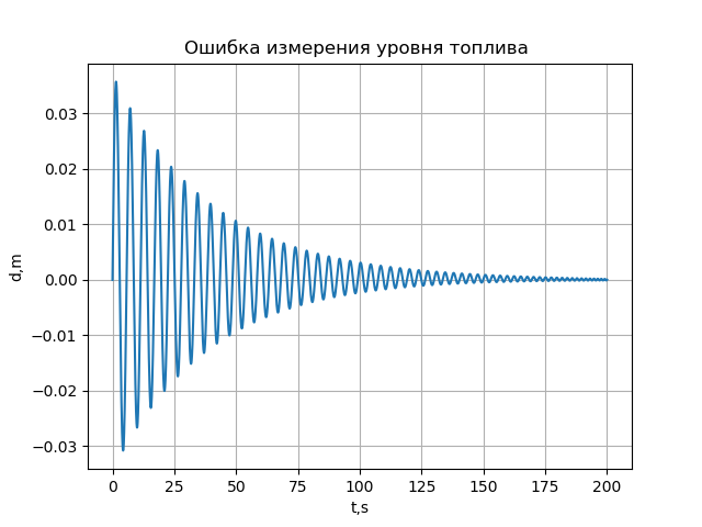
Conclusion:
This mathematical model allows us to estimate the error in measuring the level of fuel in aircraft tanks.
For a rocket, it is necessary to take into account the fluctuation (oscillations) of the fluid in the fuel tank of the rocket. Such fluctuations are visually shown in the publication [3].
To account for fluctuations of fuel in the tank, it is possible to consider such a simplified model:
The fluid is considered as a concentrated decreasing mass with reduced scattering and stiffness. But this is a topic for another article.
Findings:
1. The article demonstrates the capabilities of Python in numerical optimization with several limitations using the example of optimizing the shape of outboard fuel tanks.
2. The article demonstrates the possibilities of solving such equations using Python using the example of solving a non-classical differential equation.
3. The solutions obtained can also be used for educational purposes, without burdening the school or university with the purchase of Mathcad or other expensive packages.
References:
Source: https://habr.com/ru/post/350810/
All Articles