Hessian-Free Optimization with TensorFlow
Good day! I want to tell you about the optimization method known as Hessian-Free or Truncated Newton (Truncated Newton Method) and about its implementation using the library of deep learning - TensorFlow. It takes advantage of second-order optimization methods, and there is no need to read the matrix of second derivatives. This article describes the HF algorithm itself, as well as presents its work for training the direct distribution network on MNIST and XOR datasets.

Training a neural network includes minimizing the error function (loss function) in relation to its parameters (weights), of which there can be a lot. Therefore, there are many optimization methods to solve this problem.
Gradient descent is the simplest method for consistently finding the minimum of a differentiable function. (in the case of neural networks, this is a cost function). Having several options (weights of the network) and differentiating a function by them, we obtain a vector of partial derivatives or a gradient vector:
Gradient descent is fairly simple to implement and has a well-proven optimization method, but there is also a minus - it is of the first order, which means that the first derivative is taken with respect to the cost function. This in turn imposes some restrictions: we mean that our cost function locally looks like a plane and does not take into account its curvature.
')
But what if we take and use the information that the second derivatives on the value function gives us? The most well-known optimization method using second derivatives is the Newton method. The main idea of this method is to minimize the quadratic approximation of the cost function. What does this mean? Let's see.
Take the one-dimensional case. Suppose we have a function: . To find the minimum point, it is necessary to find the zero of its derivative, because we know: is at the minimum . We approximate the function decomposition in a second order Taylor series:
Consider the multidimensional case. Suppose we have a multi-dimensional function then:
As we can see, Newton's method is a second-order method and will work better than ordinary gradient descent, because instead of moving to a local minimum in each step, it moves to a global minimum if we assume that the function quadratic and second order decomposition in a Taylor series is its good approximation.
But this method has one big minus . To optimize the cost function, you must find the Hessian matrix or Hessian. . Set - vector of parameters, then:
The main idea of HF optimization is that we use the Newton method as a basis, but we use a more suitable way to minimize the quadratic function. But first we introduce the basic concepts that will be needed in the future.
Let be - network settings, where - weights matrix, the displacement vector (biases), then the network output is called: where - input vector. - loss function (loss function), - target value. And the function which we will minimize is defined as the average of the losses for all training examples (training batch) :
The conjugate gradient method (CG) is an iterative method for solving systems of linear equations of the type: .
Brief CG algorithm:
Input data: , , , - CG algorithm step
Initialization:
Repeat until the stop condition is met:
Now, using the conjugate gradient method, we can solve equation (2) and find which will minimize (1). In our case: .
Stop the CG algorithm. You can stop the conjugate gradient method based on different criteria. We will do this based on the relative progress in optimizing the quadratic function :
And now you can see that the main feature of HF optimization is that we do not need to find the Hessian directly, but we only need to find the result of his work for the vector.
As mentioned earlier, the beauty of this method is that we do not have to count the Hessian directly. It is only necessary to calculate the result of the product of the matrix of second derivatives by the vector. For this you can imagine as derived from towards :
1. The generalized Gauss-Newton matrix.
Uncertainty of the Hessian matrix is a problem for the optimization of non-convex functions, it can lead to the absence of a lower bound for a quadratic function and as a consequence, the impossibility of finding its minimum. This problem can be solved in many ways. For example, the introduction of a confidence interval will limit optimization or damping based on a penalty that adds a positive semi-definite component to the curvature matrix. and makes it positively defined.
Based on practical results, the best way to solve this problem is to use the Newton-Gauss matrix. instead of the Hesse matrix:
To find the product of the matrix by vector : , first we find the product of the Jacobian on the vector:
2. damping.
Newton's standard method can poorly optimize highly non-linear objective functions. The reason for this may be that at the initial stages of optimization, it can be very large and aggressive, since the starting point is far from the minimum point. To solve this problem, use the dumping method of changing the quadratic function. or limiting minimization in such a way that the new will lie within the limits in which will remain a good approximation .
Regularization of Tikhonov (Tikhonov regularization) or dumping of Tikhonov (Tikhonov damping). (Not to be confused with the term “regularization”, which is commonly used in the context of machine learning) This is the most well-known dumping method, which adds a quadratic penalty to the function :
3. Heuristics of Levenberg-Marquardt (Levenberg-Marquardt heuristic).
For dumping Tikhonov characteristic dynamic adjustment parameter . Change We will be according to the Levenberg-Marquardt rule, which is often used in the context of the LM method (the optimization method is an alternative to the Newton method). To use LM - heuristics, it is necessary to calculate the so-called reduction ratio:
According to Levenberg-Marquardt heuristics, we obtain the update rule :
4. The initial condition for the conjugate gradient algorithm (preconditioning).
In the context of HF optimization, we have some reversible transformation matrix with which we change so that and instead minimizing . The use of this feature in the CG algorithm requires the calculation of the transformed error vector where .
Short PCG (Preconditioned conjugate gradient) algorithm:
Input data: , , , , - CG algorithm step
Initialization:
Repeat until the stop condition is met:
Matrix selection not quite a trivial task. Also, in practice, the use of a diagonal matrix (instead of a matrix with a full rank) shows quite good results. One of the choices matrix - this is the use of a Fisher diagonal matrix (Empirical Fisher Diagonal):
5. Initialization of the CG - algorithm.
A good practice is to initialize the initial , for conjugate gradient algorithm, value found in the previous step of the HF algorithm. You can use some decay constant: . It is worth noting that the index refers to the step number of the HF algorithm, in turn, the index 0 in refers to the initial step of the CG algorithm.
Full Hessian-Free optimization algorithm:
Input data: , - dumping parameter - algorithm iteration step
Initialization:
The main HF optimization cycle:
Thus, the Hessian-Free optimization method allows solving the problems of finding the minimum of a function of high dimensionality. It does not require finding the Hesse matrix directly.
The theory is certainly good, but let's try to implement this optimization method in practice and see what happens. For writing the HF algorithm, I used Python and the TensorFlow library of deep learning. After that, as a performance check, I trained a direct distribution network with several layers on XOR and MNIST datasets, using the HF method for optimization.
Implementation (creating a calculation graph TensorFlow) for the conjugate gradient method.
Code to calculate the matrix to find the preconditioning condition below. At the same time, since Tensorflow summarizes the result of calculating gradients across the entire set of training examples, we had to distort a bit to get the gradient separately for each example, which affected the numerical stability of the solution. Therefore, the use of preconditioning is possible, as they say, at your own peril and risk.
The calculation of the product of the Hessian on the vector (4). It uses dumping Tikhonov (6).
When I wanted to use the generalized Newton-Gauss matrix (5), I ran into a small problem. Namely, TensorFlow cannot count Jacobian’s vector work as another Theano deep learning framework does (there is a Rop function specifically designed for this in Theano). I had to do an analog operation in TensorFlow.
And then implement the product of the generalized Newton-Gauss matrix by a vector.
The function of the main learning process is presented below. First, the quadratic function is minimized with the help of CG / PCG, then the main update of the weights of the network occurs. The dumping parameter is also adjusted based on the Levenberg-Marquardt heuristics.
We are testing an HF optimizer written for this, we will use a simple example with XOR dataset and more complex with MNIST dataset. In order to see the learning outcomes and visualize some information, we use TesnorBoard. I would also like to note that we have a rather complicated graph of calculations TensorFlow.
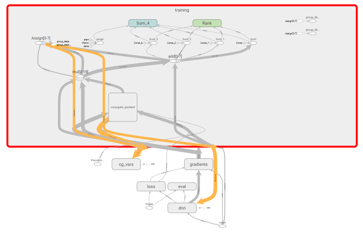
TensorFlow calculation graph.
Architecture and network training on XOR.
Create a simple network of size: 2 input neurons, 2 hidden and 1 output. We will use sigmoid as an activation function. As a loss function, use log-loss.
Now we compare the learning results using HF optimization (with the Hessian matrix), HF optimization (with the Newton-Gauss matrix) and the usual gradient descent with the learning speed parameter equal to 0.01. The number of iterations is 100.
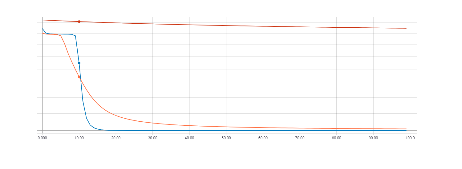
Loss for gradient descent (red line). Loss for HF optimization with Hesse matrix (orange line). Loss for HF optimization with Newton-Gauss matrix (blue line).
In this case, it is clear that the HF optimization with the use of the Newton-Gauss matrix converges most quickly, but for the gradient descent of the 100 iteration it turned out to be very small. In order for the loss function during the gradient descent to be comparable to the HF optimization, it took about 100,000 iterations .
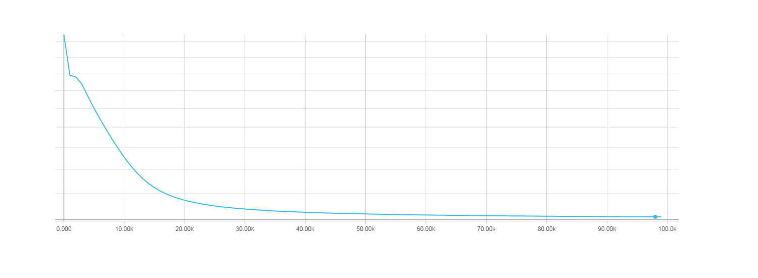
Loss for gradient descent, 100,000 iterations.
Network Architecture and Training on MNIST Dataset.
To solve the problem of recognizing handwritten numbers, create a network of size: 784 input neurons, 300 hidden and 10 output. As a loss function, we will use cross-entropy. The size of the mini batch filed during training is 50.
Just as in the case of XOR, we compare the learning outcomes using HF optimization (with the Hessian matrix), HF optimization (with the Newton-Gauss matrix) and the usual gradient descent with the learning speed parameter equal to 0.01. The number of iterations is 200, i.e. if the size of the mini batch is 50, then 200 is not a complete epoch (not all examples from the training sample are used). I did this in order to test everything faster, but even this shows a general trend.
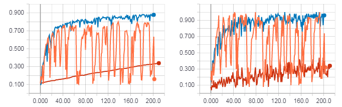
The figure on the left is the accuracy for the test sample. The figure on the right is the accuracy for the training sample. Accuracy for gradient descent (red line). Accuracy for HF optimization with Hesse matrix (orange line). Accuracy for HF optimization with Newton-Gauss matrix (blue line).
Loss for gradient descent (red line). Loss for HF optimization with Hesse matrix (orange line). Loss for HF optimization with Newton-Gauss matrix (blue line).
As you can see from the figures above, HF optimization with the Hesse matrix is not very stable, but in the end it will still converge when learning from several eras. The best result is shown by the HF optimization with the Newton-Gauss matrix.
One complete epoch of learning. The figure on the left is the accuracy for the test sample. The figure on the right is the accuracy for the training sample. Accuracy for gradient descent (turquoise line). Loss for HF optimization with Newton-Gauss matrix (pink line).
One complete epoch of learning. Loss for gradient descent (turquoise line). Loss for HF optimization with Newton-Gauss matrix (pink line).
When using the method of conjugate gradients with the initial condition for the algorithm of conjugate gradients (preconditioning), the calculations themselves slowed down and converged no faster than with the usual CG.

Loss for HF optimization using PCG algorithm.
From all these graphs, it can be noted that HF optimization using the Newton-Gauss matrix and the standard conjugate gradient method showed the best result.
The full code can be viewed on GitHub .
As a result, an implementation of the HF algorithm in Python was created using the TensorFlow library. During the creation, I ran into some problems with the implementation of the main features of the algorithm, namely: support for the Newton-Gauss matrix and preconditioning. This was due to the fact that all the same TensorFlow is not such a flexible library as we would like and is not much intended for research. For experimental purposes, it is still better to use Theano, as it gives more freedom. But I initially decided for myself to do all this with the help of TensorFlow. The program was tested and it was possible to see that the best results are obtained by the HF algorithm using the Newton-Gauss matrix. Using the same initial condition for the algorithm of conjugate gradients (preconditioning) gave unstable numerical results and slowed down the calculations, but it seems to me that this was due to TensorFlow (for the implementation of preconditioning, it had to be greatly distorted).
In this article, the theoretical aspects of Hessian - Free optimization are described quite briefly, so that you can understand the basic essence of the algorithms. If a more detailed description of the material is needed, below are sources from which I took the basic theoretical information, on the basis of which I made the Python implementation of the HF method.
1) Training Deep and Recurrent Networks with Hessian-Free Optimization (James Martens and Ilya Sutskever, University of Toronto) - a full description of HF - optimization.
2) Deep learning via Hessian-free optimization (James Martens, University of Toronto) - article with the results of using HF-optimization.
3) Fast Exact Multiplication by Hessian (Barak A. Pearlmutter, Siemens Corporate Research) - a detailed description of the multiplication of the Hessian matrix by a vector.
4) A detailed description of the conjugate gradient method for the Conjugate Gradient Method without the Agonizing Pain (Jonathan Richard Shewchuk, Carnegie Mellon University) .
Little about optimization techniques
Training a neural network includes minimizing the error function (loss function) in relation to its parameters (weights), of which there can be a lot. Therefore, there are many optimization methods to solve this problem.
Gradient Descent (Gradient Descent)
Gradient descent is the simplest method for consistently finding the minimum of a differentiable function. (in the case of neural networks, this is a cost function). Having several options (weights of the network) and differentiating a function by them, we obtain a vector of partial derivatives or a gradient vector:
The gradient always points in the direction of maximum growth of the function. If we move in the opposite direction (i.e. ) then in time we will come to the minimum, which is what we needed. The simplest gradient descent algorithm:
- Initialization: randomly select parameters
- Calculate the gradient:
- Change the parameters in the direction of a negative gradient: where - some parameter learning speed (learning rate)
- Repeat the previous steps until the gradient is close enough to zero.
Gradient descent is fairly simple to implement and has a well-proven optimization method, but there is also a minus - it is of the first order, which means that the first derivative is taken with respect to the cost function. This in turn imposes some restrictions: we mean that our cost function locally looks like a plane and does not take into account its curvature.
')
Newton's Method
But what if we take and use the information that the second derivatives on the value function gives us? The most well-known optimization method using second derivatives is the Newton method. The main idea of this method is to minimize the quadratic approximation of the cost function. What does this mean? Let's see.
Take the one-dimensional case. Suppose we have a function: . To find the minimum point, it is necessary to find the zero of its derivative, because we know: is at the minimum . We approximate the function decomposition in a second order Taylor series:
We want to find such , what will be the minimum. For this we take the derivative with respect to and equate to zero:
If a quadratic function this will be the absolute minimum. If we want to find a minimum iteratively, then we take the initial and update it according to this rule:
Over time, the decision will come down to a minimum.
Consider the multidimensional case. Suppose we have a multi-dimensional function then:
Where - Hessian or matrix of second derivatives. Based on this, for updating the parameters we have the following formula:
Problems with Newton's Method
As we can see, Newton's method is a second-order method and will work better than ordinary gradient descent, because instead of moving to a local minimum in each step, it moves to a global minimum if we assume that the function quadratic and second order decomposition in a Taylor series is its good approximation.
But this method has one big minus . To optimize the cost function, you must find the Hessian matrix or Hessian. . Set - vector of parameters, then:
As you can see, the Hessian is a matrix of second derivatives of the size. and that would need to be calculated computational operations, which can be very critical for networks that have hundreds or thousands of parameters. In addition, to solve the optimization problem using the Newton method, it is necessary to find the inverse Hesse matrix , for this, it must be positively defined for all .
Positive matrix.
Matrix dimensions is called non-negative defined if it satisfies the condition: . If the strict inequality holds, then the matrix is called positive definite. An important property of such matrices is their non-singularity, i.e. existence of inverse matrix .
Hessian-free optimization
The main idea of HF optimization is that we use the Newton method as a basis, but we use a more suitable way to minimize the quadratic function. But first we introduce the basic concepts that will be needed in the future.
Let be - network settings, where - weights matrix, the displacement vector (biases), then the network output is called: where - input vector. - loss function (loss function), - target value. And the function which we will minimize is defined as the average of the losses for all training examples (training batch) :
Further, according to Newton's method, we define a quadratic function obtained by expanding into a second-order Taylor series:
Next, take the derivative with respect to from the formula above and equating it to zero we get:
To find we will use the conjugate gradient method.
Conjugate gradient method
The conjugate gradient method (CG) is an iterative method for solving systems of linear equations of the type: .
Brief CG algorithm:
Input data: , , , - CG algorithm step
Initialization:
- - error vector (residual)
- - vector of search direction (search direction)
Repeat until the stop condition is met:
Now, using the conjugate gradient method, we can solve equation (2) and find which will minimize (1). In our case: .
Stop the CG algorithm. You can stop the conjugate gradient method based on different criteria. We will do this based on the relative progress in optimizing the quadratic function :
Where - the size of the "window" for which we will consider the value of progress, . The condition for stopping is: .
And now you can see that the main feature of HF optimization is that we do not need to find the Hessian directly, but we only need to find the result of his work for the vector.
Hessian multiplication by vector
As mentioned earlier, the beauty of this method is that we do not have to count the Hessian directly. It is only necessary to calculate the result of the product of the matrix of second derivatives by the vector. For this you can imagine as derived from towards :
But the use of this formula in practice can cause a number of problems associated with the calculation with a sufficiently small . Therefore, there is a method for accurately calculating the product of a matrix by a vector. We introduce a differential operator . It denotes a derivative of some quantity. depending on , towards :
This shows that to calculate the product of the Hessian by the vector must be calculated:
Some improvements in HF optimization
1. The generalized Gauss-Newton matrix.
Uncertainty of the Hessian matrix is a problem for the optimization of non-convex functions, it can lead to the absence of a lower bound for a quadratic function and as a consequence, the impossibility of finding its minimum. This problem can be solved in many ways. For example, the introduction of a confidence interval will limit optimization or damping based on a penalty that adds a positive semi-definite component to the curvature matrix. and makes it positively defined.
Based on practical results, the best way to solve this problem is to use the Newton-Gauss matrix. instead of the Hesse matrix:
Where - Jacobian - matrix of second derivatives of loss function .
To find the product of the matrix by vector : , first we find the product of the Jacobian on the vector:
then we calculate the product of a vector on the matrix and finally multiply the matrix on .
2. damping.
Newton's standard method can poorly optimize highly non-linear objective functions. The reason for this may be that at the initial stages of optimization, it can be very large and aggressive, since the starting point is far from the minimum point. To solve this problem, use the dumping method of changing the quadratic function. or limiting minimization in such a way that the new will lie within the limits in which will remain a good approximation .
Regularization of Tikhonov (Tikhonov regularization) or dumping of Tikhonov (Tikhonov damping). (Not to be confused with the term “regularization”, which is commonly used in the context of machine learning) This is the most well-known dumping method, which adds a quadratic penalty to the function :
Where , - dumping parameter. Calculation produced as follows:
3. Heuristics of Levenberg-Marquardt (Levenberg-Marquardt heuristic).
For dumping Tikhonov characteristic dynamic adjustment parameter . Change We will be according to the Levenberg-Marquardt rule, which is often used in the context of the LM method (the optimization method is an alternative to the Newton method). To use LM - heuristics, it is necessary to calculate the so-called reduction ratio:
Where - step number HF algorithm, - the result of the CG minimization.
According to Levenberg-Marquardt heuristics, we obtain the update rule :
4. The initial condition for the conjugate gradient algorithm (preconditioning).
In the context of HF optimization, we have some reversible transformation matrix with which we change so that and instead minimizing . The use of this feature in the CG algorithm requires the calculation of the transformed error vector where .
Short PCG (Preconditioned conjugate gradient) algorithm:
Input data: , , , , - CG algorithm step
Initialization:
- - error vector (residual)
- - solution of the equation
- - vector of search direction (search direction)
Repeat until the stop condition is met:
- - solution of the equation
Matrix selection not quite a trivial task. Also, in practice, the use of a diagonal matrix (instead of a matrix with a full rank) shows quite good results. One of the choices matrix - this is the use of a Fisher diagonal matrix (Empirical Fisher Diagonal):
5. Initialization of the CG - algorithm.
A good practice is to initialize the initial , for conjugate gradient algorithm, value found in the previous step of the HF algorithm. You can use some decay constant: . It is worth noting that the index refers to the step number of the HF algorithm, in turn, the index 0 in refers to the initial step of the CG algorithm.
Full Hessian-Free optimization algorithm:
Input data: , - dumping parameter - algorithm iteration step
Initialization:
The main HF optimization cycle:
- Calculate the matrix
- Find Solving an optimization problem with CG or PCG.
- Update dumping option using the Levenberg-Marquardt heuristics
- , - parameter learning rate (learning rate)
Thus, the Hessian-Free optimization method allows solving the problems of finding the minimum of a function of high dimensionality. It does not require finding the Hesse matrix directly.
Implementing HF optimization on TensorFlow
The theory is certainly good, but let's try to implement this optimization method in practice and see what happens. For writing the HF algorithm, I used Python and the TensorFlow library of deep learning. After that, as a performance check, I trained a direct distribution network with several layers on XOR and MNIST datasets, using the HF method for optimization.
Implementation (creating a calculation graph TensorFlow) for the conjugate gradient method.
def __conjugate_gradient(self, gradients): """ Performs conjugate gradient method to minimze quadratic equation and find best delta of network parameters. gradients: list of Tensorflow tensor objects Network gradients. return: Tensorflow tensor object Update operation for delta. return: Tensorflow tensor object Residual norm, used to prevent numerical errors. return: Tensorflow tensor object Delta loss. """ with tf.name_scope('conjugate_gradient'): cg_update_ops = [] prec = None # P (9) if self.use_prec: if self.prec_loss is None: graph = tf.get_default_graph() lop = self.loss.op.node_def self.prec_loss = graph.get_tensor_by_name(lop.input[0] + ':0') batch_size = None if self.batch_size is None: self.prec_loss = tf.unstack(self.prec_loss) batch_size = self.prec_loss.get_shape()[0] else: self.prec_loss = [tf.gather(self.prec_loss, i) for i in range(self.batch_size)] batch_size = len(self.prec_loss) prec = [[g**2 for g in tf.gradients(tf.gather(self.prec_loss, i), self.W)] for i in range(batch_size)] prec = [(sum(tensor) + self.damping)**(-0.75) for tensor in np.transpose(np.array(prec))] # Ax = None if self.use_gnm: Ax = self.__Gv(self.cg_delta) else: Ax = self.__Hv(gradients, self.cg_delta) b = [-grad for grad in gradients] bAx = [b - Ax for b, Ax in zip(b, Ax)] condition = tf.equal(self.cg_step, 0) r = [tf.cond(condition, lambda: tf.assign(r, bax), lambda: r) for r, bax in zip(self.residuals, bAx)] d = None if self.use_prec: d = [tf.cond(condition, lambda: tf.assign(d, p * r), lambda: d) for p, d, r in zip(prec, self.directions, r)] else: d = [tf.cond(condition, lambda: tf.assign(d, r), lambda: d) for d, r in zip(self.directions, r)] Ad = None if self.use_gnm: Ad = self.__Gv(d) else: Ad = self.__Hv(gradients, d) residual_norm = tf.reduce_sum([tf.reduce_sum(r**2) for r in r]) alpha = tf.reduce_sum([tf.reduce_sum(d * ad) for d, ad in zip(d, Ad)]) alpha = residual_norm / alpha if self.use_prec: beta = tf.reduce_sum([tf.reduce_sum(p * (r - alpha * ad)**2) for r, ad, p in zip(r, Ad, prec)]) else: beta = tf.reduce_sum([tf.reduce_sum((r - alpha * ad)**2) for r, ad in zip(r, Ad)]) self.beta = beta beta = beta / residual_norm for i, delta in reversed(list(enumerate(self.cg_delta))): update_delta = tf.assign(delta, delta + alpha * d[i], name='update_delta') update_residual = tf.assign(self.residuals[i], r[i] - alpha * Ad[i], name='update_residual') p = 1.0 if self.use_prec: p = prec[i] update_direction = tf.assign(self.directions[i], p * (r[i] - alpha * Ad[i]) + beta * d[i], name='update_direction') cg_update_ops.append(update_delta) cg_update_ops.append(update_residual) cg_update_ops.append(update_direction) with tf.control_dependencies(cg_update_ops): cg_update_ops.append(tf.assign_add(self.cg_step, 1)) cg_op = tf.group(*cg_update_ops) dl = tf.reduce_sum([tf.reduce_sum(0.5*(delta*ax) + grad*delta) for delta, grad, ax in zip(self.cg_delta, gradients, Ax)]) return cg_op, residual_norm, dl Code to calculate the matrix to find the preconditioning condition below. At the same time, since Tensorflow summarizes the result of calculating gradients across the entire set of training examples, we had to distort a bit to get the gradient separately for each example, which affected the numerical stability of the solution. Therefore, the use of preconditioning is possible, as they say, at your own peril and risk.
prec = [[g**2 for g in tf.gradients(tf.gather(self.prec_loss, i), self.W)] for i in range(batch_size)] The calculation of the product of the Hessian on the vector (4). It uses dumping Tikhonov (6).
def __Hv(self, grads, vec): """ Computes Hessian vector product. grads: list of Tensorflow tensor objects Network gradients. vec: list of Tensorflow tensor objects Vector that is multiplied by the Hessian. return: list of Tensorflow tensor objects Result of multiplying Hessian by vec. """ grad_v = [tf.reduce_sum(g * v) for g, v in zip(grads, vec)] Hv = tf.gradients(grad_v, self.W, stop_gradients=vec) Hv = [hv + self.damp_pl * v for hv, v in zip(Hv, vec)] return Hv When I wanted to use the generalized Newton-Gauss matrix (5), I ran into a small problem. Namely, TensorFlow cannot count Jacobian’s vector work as another Theano deep learning framework does (there is a Rop function specifically designed for this in Theano). I had to do an analog operation in TensorFlow.
def __Rop(self, f, x, vec): """ Computes Jacobian vector product. f: Tensorflow tensor object Objective function. x: list of Tensorflow tensor objects Parameters with respect to which computes Jacobian matrix. vec: list of Tensorflow tensor objects Vector that is multiplied by the Jacobian. return: list of Tensorflow tensor objects Result of multiplying Jacobian (df/dx) by vec. """ r = None if self.batch_size is None: try: r = [tf.reduce_sum([tf.reduce_sum(v * tf.gradients(f, x)[i]) for i, v in enumerate(vec)]) for f in tf.unstack(f)] except ValueError: assert False, clr.FAIL + clr.BOLD + 'Batch size is None, but used '\ 'dynamic shape for network input, set proper batch_size in '\ 'HFOptimizer initialization' + clr.ENDC else: r = [tf.reduce_sum([tf.reduce_sum(v * tf.gradients(tf.gather(f, i), x)[j]) for j, v in enumerate(vec)]) for i in range(self.batch_size)] assert r is not None, clr.FAIL + clr.BOLD +\ 'Something went wrong in Rop computation' + clr.ENDC return r And then implement the product of the generalized Newton-Gauss matrix by a vector.
def __Gv(self, vec): """ Computes the product G by vec = JHJv (G is the Gauss-Newton matrix). vec: list of Tensorflow tensor objects Vector that is multiplied by the Gauss-Newton matrix. return: list of Tensorflow tensor objects Result of multiplying Gauss-Newton matrix by vec. """ Jv = self.__Rop(self.output, self.W, vec) Jv = tf.reshape(tf.stack(Jv), [-1, 1]) HJv = tf.gradients(tf.matmul(tf.transpose(tf.gradients(self.loss, self.output)[0]), Jv), self.output, stop_gradients=Jv)[0] JHJv = tf.gradients(tf.matmul(tf.transpose(HJv), self.output), self.W, stop_gradients=HJv) JHJv = [gv + self.damp_pl * v for gv, v in zip(JHJv, vec)] return JHJv The function of the main learning process is presented below. First, the quadratic function is minimized with the help of CG / PCG, then the main update of the weights of the network occurs. The dumping parameter is also adjusted based on the Levenberg-Marquardt heuristics.
def minimize(self, feed_dict, debug_print=False): """ Performs main training operations. feed_dict: dictionary Input training batch. debug_print: bool If True prints CG iteration number. """ self.sess.run(tf.assign(self.cg_step, 0)) feed_dict.update({self.damp_pl:self.damping}) if self.adjust_damping: loss_before_cg = self.sess.run(self.loss, feed_dict) dl_track = [self.sess.run(self.ops['dl'], feed_dict)] self.sess.run(self.ops['set_delta_0']) for i in range(self.cg_max_iters): if debug_print: d_info = clr.OKGREEN + '\r[CG iteration: {}]'.format(i) + clr.ENDC sys.stdout.write(d_info) sys.stdout.flush() k = max(self.gap, i // self.gap) rn = self.sess.run(self.ops['res_norm'], feed_dict) # if rn < self.cg_num_err: break self.sess.run(self.ops['cg_update'], feed_dict) dl_track.append(self.sess.run(self.ops['dl'], feed_dict)) # , (3) if i > k: stop = (dl_track[i+1] - dl_track[i+1-k]) / dl_track[i+1] if not np.isnan(stop) and stop < 1e-4: break if debug_print: sys.stdout.write('\n') sys.stdout.flush() if self.adjust_damping: feed_dict.update({self.damp_pl:0}) dl = self.sess.run(self.ops['dl'], feed_dict) feed_dict.update({self.damp_pl:self.damping}) self.sess.run(self.ops['train'], feed_dict) if self.adjust_damping: loss_after_cg = self.sess.run(self.loss, feed_dict) # (7) reduction_ratio = (loss_after_cg - loss_before_cg) / dl # - (8) if reduction_ratio < 0.25 and self.damping > self.damp_num_err: self.damping *= 1.5 elif reduction_ratio > 0.75 and self.damping > self.damp_num_err: self.damping /= 1.5 HF Optimization Testing
We are testing an HF optimizer written for this, we will use a simple example with XOR dataset and more complex with MNIST dataset. In order to see the learning outcomes and visualize some information, we use TesnorBoard. I would also like to note that we have a rather complicated graph of calculations TensorFlow.
TensorFlow calculation graph.
Architecture and network training on XOR.
Create a simple network of size: 2 input neurons, 2 hidden and 1 output. We will use sigmoid as an activation function. As a loss function, use log-loss.
# """ Log-loss cost function """ loss = tf.reduce_mean(( (y * tf.log(out)) + ((1 - y) * tf.log(1.0 - out)) ) * -1, name='log_loss') #XOR XOR_X = [[0,0],[0,1],[1,0],[1,1]] XOR_Y = [[0],[1],[1],[0]] # sess = tf.Session() hf_optimizer = HFOptimizer(sess, loss, y_out, dtype=tf.float64, use_gauss_newton_matrix=True) init = tf.initialize_all_variables() sess.run(init) # max_epoches = 100 print('Begin Training') for i in range(max_epoches): feed_dict = {x: XOR_X, y: XOR_Y} hf_optimizer.minimize(feed_dict=feed_dict) if i % 10 == 0: print('Epoch:', i, 'cost:', sess.run(loss, feed_dict=feed_dict)) print('Hypothesis ', sess.run(out, feed_dict=feed_dict)) Now we compare the learning results using HF optimization (with the Hessian matrix), HF optimization (with the Newton-Gauss matrix) and the usual gradient descent with the learning speed parameter equal to 0.01. The number of iterations is 100.
Loss for gradient descent (red line). Loss for HF optimization with Hesse matrix (orange line). Loss for HF optimization with Newton-Gauss matrix (blue line).
In this case, it is clear that the HF optimization with the use of the Newton-Gauss matrix converges most quickly, but for the gradient descent of the 100 iteration it turned out to be very small. In order for the loss function during the gradient descent to be comparable to the HF optimization, it took about 100,000 iterations .
Loss for gradient descent, 100,000 iterations.
Network Architecture and Training on MNIST Dataset.
To solve the problem of recognizing handwritten numbers, create a network of size: 784 input neurons, 300 hidden and 10 output. As a loss function, we will use cross-entropy. The size of the mini batch filed during training is 50.
with tf.name_scope('loss'): one_hot = tf.one_hot(t, n_outputs, dtype=tf.float64) xentropy = tf.nn.softmax_cross_entropy_with_logits(labels=one_hot, logits=y_out) loss = tf.reduce_mean(xentropy, name="loss") with tf.name_scope("eval"): correct = tf.nn.in_top_k(tf.cast(y_out, tf.float32), t, 1) accuracy = tf.reduce_mean(tf.cast(correct, tf.float64)) n_epochs = 10 batch_size = 50 with tf.Session() as sess: """ Initializing hessian free optimizer """ hf_optimizer = HFOptimizer(sess, loss, y_out, dtype=tf.float64, batch_size=batch_size, use_gauss_newton_matrix=True) init = tf.global_variables_initializer() init.run() # for epoch in range(n_epochs): n_batches = mnist.train.num_examples // batch_size for iteration in range(n_batches): x_batch, t_batch = mnist.train.next_batch(batch_size) hf_optimizer.minimize({x: x_batch, t: t_batch}) if iteration%10==0: print('Batch:', iteration, '/', n_batches) acc_train = accuracy.eval(feed_dict={x: x_batch, t: t_batch}) acc_test = accuracy.eval(feed_dict={x: mnist.test.images, t: mnist.test.labels}) print('Loss:', sess.run(loss, {x: x_batch, t: t_batch})) print('Target', t_batch[0]) print('Out:', sess.run(y_out_sm, {x: x_batch, t: t_batch})[0]) print(epoch, "Train accuracy:", acc_train, "Test accuracy:", acc_test) acc_train = accuracy.eval(feed_dict={x: x_batch, t: t_batch}) acc_test = accuracy.eval(feed_dict={x: mnist.test.images, t: mnist.test.labels}) print(epoch, "Train accuracy:", acc_train, "Test accuracy:", acc_test) Just as in the case of XOR, we compare the learning outcomes using HF optimization (with the Hessian matrix), HF optimization (with the Newton-Gauss matrix) and the usual gradient descent with the learning speed parameter equal to 0.01. The number of iterations is 200, i.e. if the size of the mini batch is 50, then 200 is not a complete epoch (not all examples from the training sample are used). I did this in order to test everything faster, but even this shows a general trend.
The figure on the left is the accuracy for the test sample. The figure on the right is the accuracy for the training sample. Accuracy for gradient descent (red line). Accuracy for HF optimization with Hesse matrix (orange line). Accuracy for HF optimization with Newton-Gauss matrix (blue line).
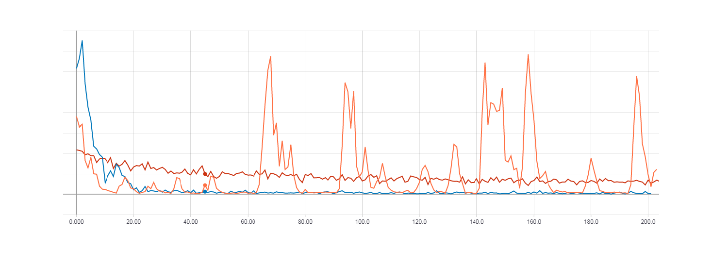
Loss for gradient descent (red line). Loss for HF optimization with Hesse matrix (orange line). Loss for HF optimization with Newton-Gauss matrix (blue line).
As you can see from the figures above, HF optimization with the Hesse matrix is not very stable, but in the end it will still converge when learning from several eras. The best result is shown by the HF optimization with the Newton-Gauss matrix.
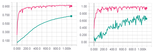
One complete epoch of learning. The figure on the left is the accuracy for the test sample. The figure on the right is the accuracy for the training sample. Accuracy for gradient descent (turquoise line). Loss for HF optimization with Newton-Gauss matrix (pink line).
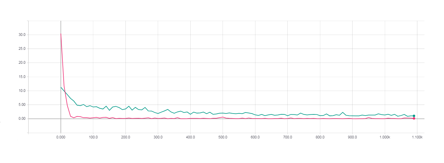
One complete epoch of learning. Loss for gradient descent (turquoise line). Loss for HF optimization with Newton-Gauss matrix (pink line).
When using the method of conjugate gradients with the initial condition for the algorithm of conjugate gradients (preconditioning), the calculations themselves slowed down and converged no faster than with the usual CG.
Loss for HF optimization using PCG algorithm.
From all these graphs, it can be noted that HF optimization using the Newton-Gauss matrix and the standard conjugate gradient method showed the best result.
The full code can be viewed on GitHub .
Results
As a result, an implementation of the HF algorithm in Python was created using the TensorFlow library. During the creation, I ran into some problems with the implementation of the main features of the algorithm, namely: support for the Newton-Gauss matrix and preconditioning. This was due to the fact that all the same TensorFlow is not such a flexible library as we would like and is not much intended for research. For experimental purposes, it is still better to use Theano, as it gives more freedom. But I initially decided for myself to do all this with the help of TensorFlow. The program was tested and it was possible to see that the best results are obtained by the HF algorithm using the Newton-Gauss matrix. Using the same initial condition for the algorithm of conjugate gradients (preconditioning) gave unstable numerical results and slowed down the calculations, but it seems to me that this was due to TensorFlow (for the implementation of preconditioning, it had to be greatly distorted).
Sources
In this article, the theoretical aspects of Hessian - Free optimization are described quite briefly, so that you can understand the basic essence of the algorithms. If a more detailed description of the material is needed, below are sources from which I took the basic theoretical information, on the basis of which I made the Python implementation of the HF method.
1) Training Deep and Recurrent Networks with Hessian-Free Optimization (James Martens and Ilya Sutskever, University of Toronto) - a full description of HF - optimization.
2) Deep learning via Hessian-free optimization (James Martens, University of Toronto) - article with the results of using HF-optimization.
3) Fast Exact Multiplication by Hessian (Barak A. Pearlmutter, Siemens Corporate Research) - a detailed description of the multiplication of the Hessian matrix by a vector.
4) A detailed description of the conjugate gradient method for the Conjugate Gradient Method without the Agonizing Pain (Jonathan Richard Shewchuk, Carnegie Mellon University) .
Source: https://habr.com/ru/post/350794/
All Articles