R means regression

Statistics has recently received powerful PR support from newer and more noisy disciplines - Machine Learning and Big Data . Those who seek to ride this wave must make friends with the regression equations . It is desirable not only to learn 2-3 receivers and pass the exam, but to be able to solve problems from everyday life: to find the relationship between variables, and ideally to be able to distinguish the signal from the noise.

For this purpose we will use a programming language and the R development environment, which is perfectly adapted to such tasks. At the same time, let's check what the rating of Habrapost depends on the statistics of its own articles.

Introduction to Regression Analysis

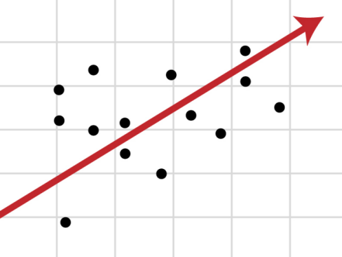
If there is a correlation $$$F (y) = F (x, y)$between variables y and x , it is necessary to determine the functional relationship between the two quantities. Dependence of the mean $$$\ mu_ {1y} = f (x)$called y regression x .

The basis of the regression analysis is the least squares method (OLS) , according to which the function is taken as the regression equation $$$y = f (x)$such that the sum of the squared differences $$$s = \ sum_ {i = 1} ^ n [y_i - f (x) _i] ^ 2$is minimal.

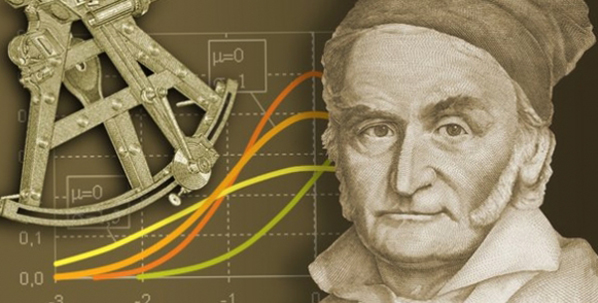
Karl Gauss discovered, or rather recreated, the MNC at the age of 18, but the results were first published by Legendre in 1805. According to unconfirmed data, the method was known in ancient China, from where it migrated to Japan and only then came to Europe. The Europeans did not make this secret and successfully launched into production, finding with it the trajectory of the dwarf planet Ceres in 1801.

Type of function $$$y = f (x)$As a rule, it is determined in advance, and with the help of the OLS, the optimal values ​​of the unknown parameters are selected. Scattering metric values $$$y_i$around regression $$$f (x)$is the variance.

$$

$$D = \ frac {1} {n-k} \ sum_ {i = 1} ^ n [y_i - f (x) _i] ^ 2$$

• k is the number of coefficients in the system of regression equations.

The most commonly used model is linear regression, and all non-linear dependencies $$$y = f (x)$lead to a linear form with the help of algebraic tweaks, various transformations of the variables y and x .

Linear regression

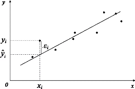
The linear regression equations can be written as

$$

$$y = x_1 + \ beta_1 + ... x_k \ beta_k + \ epsilon.$$

In the matrix view it looks smooth.

$$

$$y = X \ beta + \ epsilon$$

• y is the dependent variable;
• x is an independent variable;
• β - coefficients that must be found using the OLS;
• ε is the error, unexplained error and deviation from linear dependence;

Random value $$$y_i$can be interpreted as the sum of two terms:

• $$$y_i$- total dispersion (TSS).
• $$$\ widehat {y_i}$- explained part of the variance (ESS).
• $$$\ epsilon_i = y_i - \ widehat {y_i}$- residual part of the dispersion (RSS).

Another key concept is the correlation coefficient R ² .

$$

$$R ^ 2 = 1 - ESS / TSS$$

Linear regression constraints

In order to use the linear regression model, some assumptions are needed regarding the distribution and properties of variables.

1. Linearity , actually. Increasing or decreasing the vector of independent variables by k times leads to a change in the dependent variable also k times.
2. The matrix of coefficients has full rank , that is, the vectors of independent variables are linearly independent.
3. Exogenous independent variables - $$$E [\ epsilon_i | x_ {j1}, x_ {j2}, ... x_ {jk}] = 0$. This requirement means that the mathematical expectation of the error can in no way be explained using independent variables.
4. Dispersion homogeneity and lack of autocorrelation . Each ε _i has the same and final dispersion σ ² and does not correlate with the other ε _i . This significantly limits the applicability of the linear regression model, it is necessary to make sure that the conditions are met, otherwise the detected relationship of variables will be incorrectly interpreted.

How to find that the above conditions are not met? Well, firstly, quite often it can be seen with the naked eye on the chart.

Dispersion heterogeneity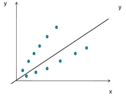

With increasing dispersion with increasing independent variable, we have a funnel-shaped graph.

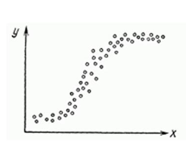
Nonlinear regression in some cases is also fashionable to see on the graph quite clearly.

Nevertheless, there are quite strict formal ways to determine whether the conditions of linear regression are met, or are violated.

• Autocorrelation is verified by Durbin-Watson statistics (0 ≤ d ≤ 4). If there is no autocorrelation, the values ​​of the criterion d≈2, with a positive autocorrelation d≈0, with a negative - d≈4.
• Dispersion Heterogeneity - White Test , $$$\ chi {^ 2} _ {obs} = nR ^ 2$at $$$\ chi {^ 2} _ {obs}> \ chi {^ 2} _ {\ alpha; m-1}$the null hypothesis is rejected and the presence of inhomogeneous dispersion is stated. Using the same $$$\ chi {^ 2} _ {obs}$you can still apply the test Broysh-Pagan .
• Multicollinearity - violation of the condition of the absence of a reciprocal linear relationship between independent variables. To check often use VIFs (Variance Inflation Factor).

$$

$$VIF_j = \ frac {1} {1-R {^ 2} _j}$$

In this formula $$$R {^ 2} _j$- the coefficient of mutual determination between $$$X_j$and other factors. If at least one of the VIFs is> 10, it is quite reasonable to assume the presence of multicollinearity.

Why is it important for us to comply with all the above conditions? It is all a matter of the Gauss-Markov Theorem , according to which the OLS estimate is accurate and effective only if these restrictions are observed.

How to overcome these limitations

Violation of one or more restrictions is not a sentence yet.

1. Regression nonlinearity can be overcome by transforming variables, for example, through the natural logarithm function ln .
2. In the same way, it is possible to solve the problem of non-uniform dispersion, using ln , or sqrt transformations of the dependent variable, or using weighted OLS.
3. To eliminate the problem of multicollinearity, the method of eliminating variables is used. Its essence is that the highly correlated explanatory variables are eliminated from the regression , and it is re-evaluated. The criterion for selecting the variables to be excluded is the correlation coefficient. There is another way to solve this problem, which is to replace the variables in which multicollinearity is inherent in their linear combination . This whole list is not exhausted; there is also stepwise regression and other methods.

Unfortunately, not all violations of the conditions and defects of the linear regression can be eliminated using the natural logarithm. If there is an autocorrelation of perturbations for example, then it is better to step back and build a new and better model.

Linear regression of pluses on Habré

So, quite theoretical baggage and you can build the model itself.
I have long been curious about what that very green figure depends on, which indicates the rating of the post on Habré. Having collected all the available statistics of my own posts, I decided to drive it through the linear regression model.

Loads data from tsv file.

 > hist <- read.table("~/habr_hist.txt", header=TRUE) > hist 

 points reads comm faves fb bytes 31 11937 29 19 13 10265 93 34122 71 98 74 14995 32 12153 12 147 17 22476 30 16867 35 30 22 9571 27 13851 21 52 46 18824 12 16571 44 149 35 9972 18 9651 16 86 49 11370 59 29610 82 29 333 10131 26 8605 25 65 11 13050 20 11266 14 48 8 9884 ... 

• points - Article rating
• reads - The number of views.
• comm - The number of comments.
• faves - Added to bookmarks.
• fb - Shared on social networks (fb + vk).
• bytes - The length in bytes.

Multicollinearity check.

 > cor(hist) points reads comm faves fb bytes points 1.0000000 0.5641858 0.61489369 0.24104452 0.61696653 0.19502379 reads 0.5641858 1.0000000 0.54785197 0.57451189 0.57092464 0.24359202 comm 0.6148937 0.5478520 1.00000000 -0.01511207 0.51551030 0.08829029 faves 0.2410445 0.5745119 -0.01511207 1.00000000 0.23659894 0.14583018 fb 0.6169665 0.5709246 0.51551030 0.23659894 1.00000000 0.06782256 bytes 0.1950238 0.2435920 0.08829029 0.14583018 0.06782256 1.00000000 

Contrary to my expectations, the greatest return is not on the number of article views, but on comments and publications in social networks . I also believed that the number of views and comments would have a stronger correlation, but the dependence is quite moderate - there is no need to exclude any of the independent variables.

Now the model itself, we use the function lm .

 regmodel <- lm(points ~., data = hist) summary(regmodel) Call: lm(formula = points ~ ., data = hist) Residuals: Min 1Q Median 3Q Max -26.920 -9.517 -0.559 7.276 52.851 Coefficients: Estimate Std. Error t value Pr(>|t|) (Intercept) 1.029e+01 7.198e+00 1.430 0.1608 reads 8.832e-05 3.158e-04 0.280 0.7812 comm 1.356e-01 5.218e-02 2.598 0.0131 * faves 2.740e-02 3.492e-02 0.785 0.4374 fb 1.162e-01 4.691e-02 2.476 0.0177 * bytes 3.960e-04 4.219e-04 0.939 0.3537 --- Signif. codes: 0 '***' 0.001 '**' 0.01 '*' 0.05 '.' 0.1 ' ' 1 Residual standard error: 16.65 on 39 degrees of freedom Multiple R-squared: 0.5384, Adjusted R-squared: 0.4792 F-statistic: 9.099 on 5 and 39 DF, p-value: 8.476e-06 

In the first line we set the parameters of the linear regression. Line points ~. defines the dependent variable points and all other variables as regressors. You can define one single independent variable in terms of points ~ reads , a set of variables - points ~ reads + comm .

We now turn to the decoding of the results.

• Intercept - If our model is represented as $$$\ beta_0 + \ beta_1 * x + \ epsilon$, so then $$$\ beta_0$- the point of intersection of the line with the axis of coordinates, or intercept .
• R-squared - The coefficient of determination indicates how close is the relationship between the regression factors and the dependent variable; this is the ratio of the sum of squares of perturbations explained to the unexplained. The closer to 1, the more pronounced the dependence .
• Adjusted R-squared - Problem with $$$R ^ 2$in that it grows in any way with a number of factors, therefore a high value of this coefficient can be deceptive when there are many factors in the model. In order to remove this property from the correlation was invented.
• F-statistic - Used to assess the significance of the regression model as a whole, is the ratio of the explicable variance to the unexplained. If the linear regression model is constructed successfully, then it explains a significant part of the variance, leaving a small part in the denominator. The higher the value of the parameter, the better .
• t value - A criterion based on t . The value of a parameter in a linear regression indicates the significance of a factor; it is generally accepted that when t > 2 factor is significant for the model.
• p value - This is the probability of the nullity of the hypothesis, which states that independent variables do not explain the dynamics of the dependent variable. If the value of p value below the threshold level (.05 or .01 for the most demanding), then the null hypothesis is false. The lower the better .

$$

$$F = \ frac {RSS * (m-1)} {ESS * (n-m)} = \ frac {R ^ 2} {1-R ^ 2} * \ frac {m-1} {n-m}$$

You can try to slightly improve the model by smoothing non-linear factors: comments and posts on social networks. Replace the values ​​of the variables fb and comm their powers.

 > hist$fb = hist$fb^(4/7) > hist$comm = hist$comm^(2/3) 

Check the values ​​of the linear regression parameters.

 > regmodel <- lm(points ~., data = hist) > summary(regmodel) Call: lm(formula = points ~ ., data = hist) Residuals: Min 1Q Median 3Q Max -22.972 -11.362 -0.603 7.977 49.549 Coefficients: Estimate Std. Error t value Pr(>|t|) (Intercept) 2.823e+00 7.305e+00 0.387 0.70123 reads -6.278e-05 3.227e-04 -0.195 0.84674 comm 1.010e+00 3.436e-01 2.938 0.00552 ** faves 2.753e-02 3.421e-02 0.805 0.42585 fb 1.601e+00 5.575e-01 2.872 0.00657 ** bytes 2.688e-04 4.108e-04 0.654 0.51677 --- Signif. codes: 0 '***' 0.001 '**' 0.01 '*' 0.05 '.' 0.1 ' ' 1 Residual standard error: 16.21 on 39 degrees of freedom Multiple R-squared: 0.5624, Adjusted R-squared: 0.5062 F-statistic: 10.02 on 5 and 39 DF, p-value: 3.186e-06 

As you can see, in general, the responsiveness of the model has increased, the parameters have been tightened and become more silky , F- increased, as did the .

Check whether the conditions of applicability of the linear regression model? The Durbin-Watson test checks for autocorrelation of disturbances.

 > dwtest(hist$points ~., data = hist) Durbin-Watson test data: hist$points ~ . DW = 1.585, p-value = 0.07078 alternative hypothesis: true autocorrelation is greater than 0 

And finally, test the dispersion heterogeneity using the test Broysh-Pagan.

 > bptest(hist$points ~., data = hist) studentized Breusch-Pagan test data: hist$points ~ . BP = 6.5315, df = 5, p-value = 0.2579 

Finally

Of course, our linear regression model of the Habra Topics ranking was not the most successful. We managed to explain no more than half the variability of the data. Factors need to be repaired to get rid of inhomogeneous dispersion, with autocorrelation is also unclear. In general, data is not enough for any serious assessment.

But on the other hand, it is good. Otherwise, any hastily written troll post on Habré would automatically gain a high rating, and this is fortunately not the case.

Used materials

1. Beginners Guide to Regression Analysis and Plot Interpretations
2. Methods of correlation and regression analysis
3. Kobzar A. I. Applied mathematical statistics. - M .: Fizmatlit, 2006.
4. William H. Green Econometric Analysis