Background removal using deep learning

Translation Background removal with deep learning .

For the last several years of work in the field of machine learning, we have wanted to create real products based on machine learning.
')
A few months ago, after passing the excellent course Fast.AI , the stars coincided, and we had the opportunity. Modern advances in technology of deep learning have made it possible to accomplish much of what previously seemed impossible, new tools appeared that made the implementation process more accessible than ever.

We set the following goals:

1. Improve our skills with deep learning.
2. Improve our skills in introducing products based on AI.
3. Create a useful product with market prospects.
4. Have fun (and help our users have fun).
5. Exchange experience.

Given the above, we studied ideas that:

1. No one has yet been able to implement (or implement properly).
2. They will not be too complicated in planning and implementation - we spent 2-3 months working on a project with a workload of 1 working day per week.
3. They will have a simple and attractive user interface - we wanted to make a product that people will use, and not just for demonstration purposes.
4. They will have available data for training - as any machine learning specialist knows, sometimes data is more expensive than an algorithm.
5. They will use advanced deep learning methods (which have not yet been marketed by Google, Amazon or their friends on cloud platforms), but not too advanced (so that we can find a few examples on the Internet).
6. Will have the potential to achieve a result sufficient to bring the product to market.

Our early assumptions were to take on some kind of medical project, since this area is very close to us, and we felt (and still feel) that there are a huge number of topics suitable for deep learning. However, we realized that we would encounter problems in collecting data and, possibly, legality and regulation, which contradicted our desire not to complicate the task ourselves. Therefore, we decided to stick with plan B - to make a product for removing background in images.

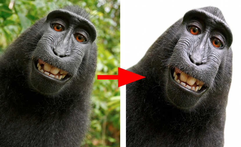
Background removal is a task that is easy to perform manually, or almost manually (Photoshop, and even Power Point have such tools) if you use some kind of “marker” and border detection technology, see an example . However, fully automated background removal is a rather difficult task, and, as far as we know, there is still no product that has achieved acceptable results (although there are those who are trying ).

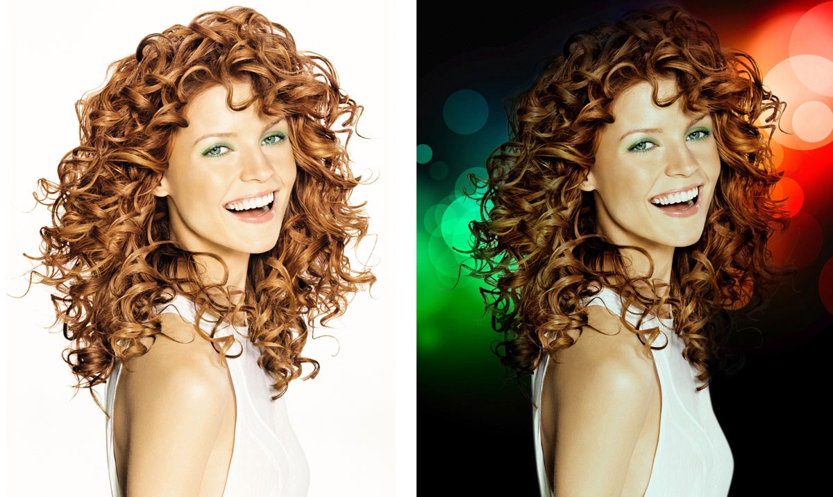
What background will we delete? This question turned out to be important, because the more specific the model is in terms of objects, angles, etc., the higher the quality of the background and foreground separation will be. When we started our work, we thought broadly: a comprehensive background removal tool that automatically identifies the foreground and background in each type of image. But after learning our first model, we realized that it was better to focus our efforts on a specific set of images. Therefore, we decided to focus on selfies and portraits of people.


Removing the background on a photo (almost) of a person.

Selfie is an image:

• with a characteristic and foreground oriented (one or more “people”), which guarantees us a good separation between the object (face + upper body) and the background,
• and also with a constant angle and always the same object (person).

Considering these statements, we started research and implementation, having spent many hours on training in order to create an easy-to-use background removal service with one click.

The main part of our work was to train the model, but we could not afford to underestimate the importance of proper implementation. Good segmentation models are still not as compact as image classification models (for example, SqueezeNet ), and we actively explored deployment options on both the server side and the browser side.

If you want to read more about the implementation process of our product, you can read our posts about the implementation on the server side and on the client side.

If you want to learn about the model and its learning process, continue to read here.

Semantic segmentation

When studying the tasks of deep learning and computer vision, resembling the tasks before us, it is easy to understand that the best option for us is the task of semantic segmentation .

There are other strategies, such as dividing by depth , but they seemed not mature enough for our purposes.

Semantic segmentation is a well-known computer vision task, one of the three most important, along with the classification and detection of objects. Segmentation, in fact, is the task of classification, in the sense of the distribution of each pixel into classes. Unlike image classification or image detection models, the segmentation model does demonstrate some “understanding” of images, that is, not only says “there is a cat in this image”, but also indicates at the pixel level where this cat is.

So how does segmentation work? To better understand, we will need to explore some of the early work in this area.

The very first idea was to adapt some of the early classification networks, such as VGG and Alexnet. VGG (Visual Geometry Group) was an advanced model for image classification in 2014, and even today it is very useful due to its simple and clear architecture. When studying the early layers of VGG, it can be noted that high activation is inherent in the categorization. Deeper layers have even stronger activation, however, they are terrible in nature due to repeated pooling action. With all this in mind, it has been suggested that the method of classification can also be used to search / segmentation of an object, with some changes.

Early results of semantic segmentation appeared along with classification algorithms. In this post you can see some rough segmentation results obtained using VGG:



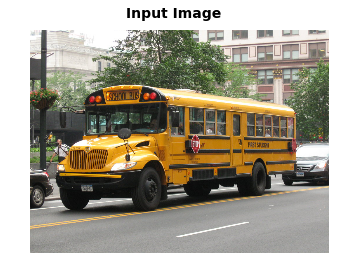
The results of the deeper layers:


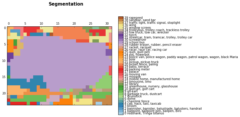
The segmentation of the bus image, light purple (29) - is the class of the school bus.

After bilinear resampling:



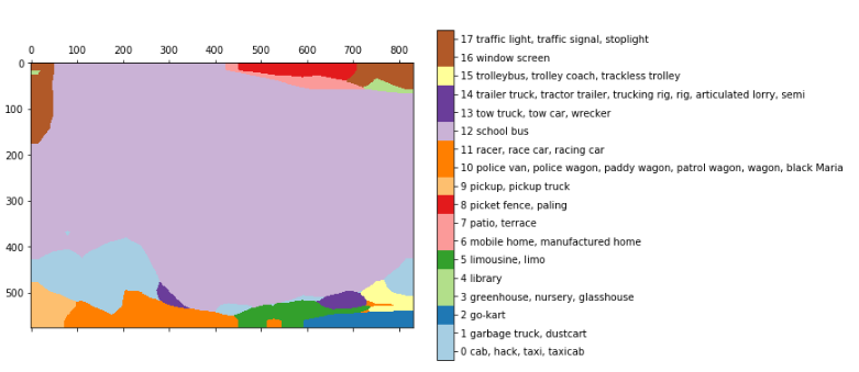
These results are obtained from a simple transformation (or maintenance) of a fully connected layer into its original form, retaining its spatial characteristics and obtaining a complete convolutional neural network. In the example above, we load the image 768 * 1024 into VGG and get the layer 24 * 32 * 1000. 24 * 32 is the image after pooling (32 each), and 1000 is the number of image-net classes from which we can get the above segmentation

To improve prediction, researchers simply used a bilinear resampling layer.

In the work of FCN, the authors improved the above idea. They put together several layers to produce more intense interpretations, which they called FCN-32, FCN-16 and FCN-8, according to the frequency of resampling:



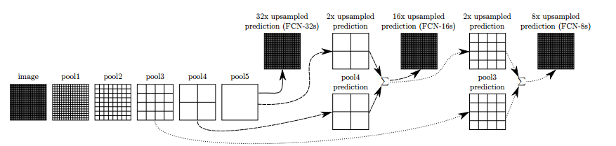
Adding some bandwidth connections (skip connections) between layers made it possible to predict with encoding more fine details of the original image. Further training further improved results.

This method proved to be not as bad as one might think, and proved that semantic segmentation with deep learning really does have potential.


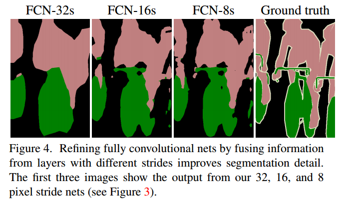
FCN results.

FCN uncovered the concept of segmentation, and researchers were able to test different architectures for this task. The basic idea remained unchanged: the use of well-known architectures, resampling and throughput connections are still present in more recent models.

You can read about achievements in this area in several good posts: here , here and here . You may also notice that most architectures have an “encoder-decoder” scheme.

Returning to our project

After some research, we stopped at three models available to us: FCN, Unet and Tiramisu - these are very deep architectures of the "encoder-decoder" type. We also had some thoughts on the mask-RCNN method, but its implementation was outside the scope of our project.

FCN did not seem relevant, since its results were not as good as we wanted (even as a starting point), but the other two models showed good results: the main advantages of Unet and Tiramisu with CamVid were their compactness and speed. Unet was pretty easy to implement (we used keras), but Tiramisu was also quite realizable. To start somewhere, we used the good Tiramisu implementation described in the last lesson of the Jeremy Howard in- depth training course .

We started to teach these two models on some datasets. It must be said that after we first tried Tiramisu, its results had much greater potential for us, since the model could capture the sharp edges of the image. Unet, in turn, was not good enough, and the results looked a bit blurry.


Blur Unet results.

Data

Having defined the model, we began to look for suitable datasets. Data for segmentation is not as common as data for classification, or even for detection. In addition, we could not index images manually. The most popular datasets for segmentation were: COCO , which includes about 80 thousand images in 90 categories, VOC pascal with 11 thousand images in 20 classes, and more recent ADE20K .

We decided to work with COCO because it includes many more images of the “person” class that interested us.

Considering our task, we have thought about whether we will use only relevant for us images or more “common” data. On the one hand, using a more general dataset with a large number of images and classes will allow the model to cope with more scenarios and tasks. On the other hand, training for one night allowed us to process ~ 150 thousand images. If we provide the entire COCO dataset to the model, then it will see each image twice (on average), so it’s better to cut it a little. In addition, our model will be better sharpened by our task.

Another point worth mentioning is that the Tiramisu model was originally trained in the CamVid dataset, which has some flaws, the main one of which is a strong monotony of images: photos of roads taken from cars. As you can understand, training on such a dataset (even if it contains people) did not benefit us, so after some trials we moved on.


Images from CamVid.

Dataset COCO comes with a fairly simple API that allows us to know exactly which objects are on which image (according to 90 predefined classes).

After some experiments, we decided to dilute the dataset: at first, only the images with the person were filtered out, leaving 40 thousand pictures. Then they discarded all the images with several people, leaving only photos with 1-2 people, because our product is intended for such situations. Finally, we left only the images in which a person occupies 20% - 70% of the area, deleting images with too small a person or with some strange monsters (unfortunately, we were not able to remove all of them). Our final dataset consisted of 11,000 images, which we felt were sufficient at this stage.


Left: the right image. Center: Too many participants. Right: The object is too small.

Tiramisu model

Although the full name of the Tiramisu model ("100 layers of Tiramisu") implies a giant model, in fact it is quite economical and uses only 9 million parameters. For comparison, the VGG16 uses over 130 million parameters.

The Tiramisu model is based on DenseNet, a fresh image classification model in which all layers are interconnected. In addition, throughput connections are added to the oversampling layers in Tiramisu, as in Unet.

If you remember, this architecture is consistent with the idea presented in FCN: using the classification architecture, resampling, and adding bandwidth connections for optimization.


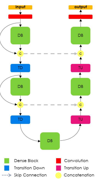
This is the architecture of Tiramisu.

The DenseNet model can be viewed as a natural evolution of the Resnet model, but instead of “memorizing” each layer only up to the next layer, Densenet remembers all layers in the entire model. Such connections are called highway connections. This leads to an increase in the number of filters, called the “growth rate”. Tiramisu has a growth rate of 16, that is, with each layer we add 16 new filters until we reach layers of 1072 filters. You could expect 1600 layers, because this is a 100-layer Tiramisu model, however, the resampled layers discard some filters.


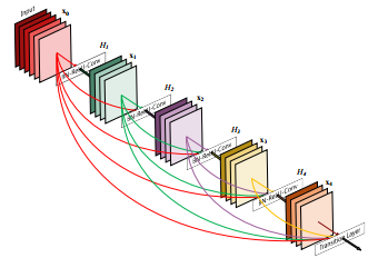
Densenet's model schema — early filters are going on the stack throughout the entire model.

Training

We trained our model according to the schedule described in the original document: standard cross-entropy loss, RMSProp optimizer with a 1E-3 learning coefficient and a slight weakening. We divided our 11 thousand images into three parts: 70% for training, 20% for testing and 10% for testing. All images below are taken from our test dataset.

In order for our training schedule to coincide with that given in the original document, we set the sampling period at a level of 500 images. This also allowed us with each improvement of the results to periodically save the model, since we trained it on much more data than in the document (the CamVid datas used in this article contained less than 1,000 images).

In addition, we trained our model using only two classes: background and person, and there were 12 classes in the source document. At first we tried to teach COCO dataset on some classes, however, we noticed that this does not lead to an improvement in the results.

Data problems

Some disadvantages of dataset lowered our assessment:

• Animals Our model sometimes segmented animals. This, of course, leads to a low IoU (intersection over union, the ratio of the intersection to the union). Adding animals to the main class or to a separate one would probably affect our results.
• Body parts Since we programmatically filtered our dataset, we were unable to determine whether a person’s class is really a person, not a part of the body, for example, a hand or a foot. These images were not of interest to us, but still appeared here and there.
  
  
  
  
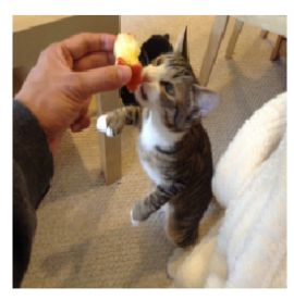
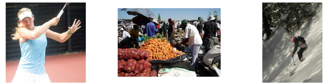
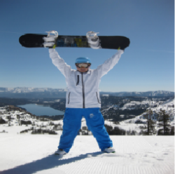
  Animal, body part, portable object.
• Portable objects . Many images in dataset are related to sports. Baseball bats, tennis rackets and snowboards were everywhere. Our model was somehow “confused”, not understanding how to segment it. As in the case of animals, in our opinion, adding them as part of the main class (or as a separate class) would help improve the performance of the model.
  
  
  
  
  Sports image with object.
• Rough control data (ground truth) . COCO dataset was annotated not pixel-by-pixel, but with the help of polygons. Sometimes this is enough, but in some cases the control data is too “rough”, which may prevent the model from learning the finer points.
  
  
  
  
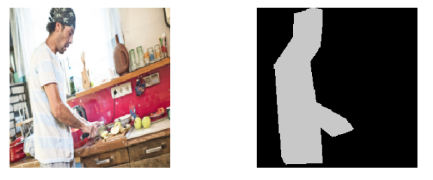
  The image itself and (very) rough control data.

results

Our results were satisfactory, although not perfect: we achieved an IoU of 84.6 on our test dataset, while the current achievement is a value of 85 IoU. However, the specific value varies depending on dataset and class. There are classes that are inherently easier to segment, for example, houses or roads, where most models easily achieve results in 90 IoU. More difficult classes are trees and people, on which most models achieve results around 60 IoU. Therefore, we helped our network focus on one class and limited types of photos.

We still do not feel that our work is “ready for release,” as we would like, but we believe that it’s time to stop and discuss our achievements, since about 50% of the photos will give good results.

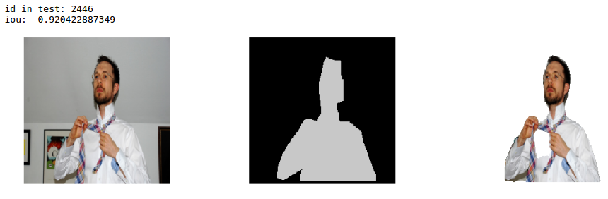
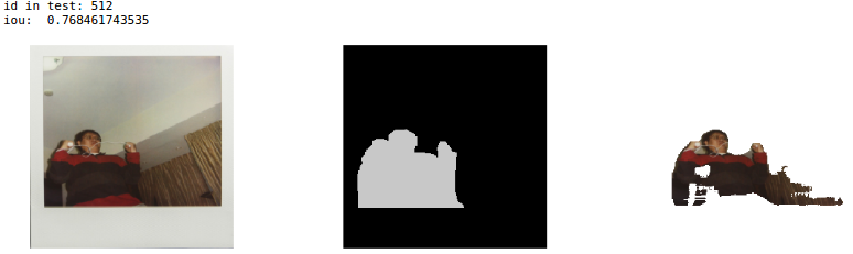
Here are some good examples that will help you to feel the possibilities of the application:


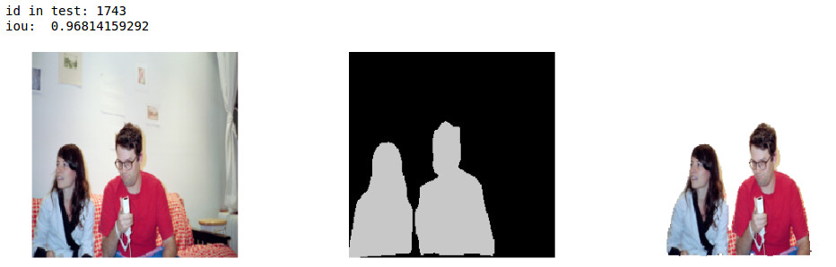
Image - control data - our results (from our test dataset).

Debugging and Logging

Debugging is a very important part of learning neural networks. At the beginning of our work it was very tempting to get down to business right away - take data and a network, start learning and see what happens. However, we found that it is extremely important to track each step, exploring the results at each stage.

Here are the frequently encountered difficulties and our solutions:

1. Early problems . Model can not begin to learn. This may be due to an internal problem or a preprocessing error, for example, if you forget to normalize some pieces of data. In any case, a simple visualization of the results can be very useful. Here is a good post on this topic.
2. Debugging the network itself . In the absence of serious problems, learning begins with predetermined losses and metrics. In segmentation, the main criterion is IoU - the ratio of the intersection to the union. It took us several sessions to start using IoU as the main criterion for our models (and not the loss of cross-entropy). Another useful practice has been to display the prediction of our model at each sampling period. Here is a good article on debugging machine learning models. Please note that IoU is not a standard metric / loss in keras, but you can easily find it on the Internet, for example, here . We also used this gist for scheduling losses and some prediction in each sampling period.
3. Control of machine learning versions . There are many parameters in teaching a model, and some of them are quite complex. I must say that we still have not found the ideal method, except that we enthusiastically fixed all our configurations (and automatically saved the best models with the callback call, see below).
4. Debug tool After doing all of the above, we were able to analyze our work at every step, but not without difficulty. Therefore, the most important step was to combine the above steps and upload the data to Jupyter Notebook (a tool for creating analytical reports), which allowed us to easily load each model and each image, and then quickly study the results. Thus, we were able to see the differences between the models and detect pitfalls and other problems.

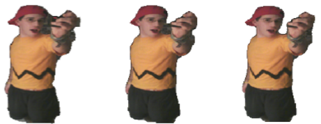
Here are examples of improving our model, achieved through parameter settings and additional training:



To save the model with the best IoU result (to simplify the work, Keras allows you to make very good callbacks ):

callbacks = [keras.callbacks.ModelCheckpoint(hist_model, verbose=1,save_best_only =True, monitor= 'val_IOU_calc_loss'), plot_losses]

In addition to the usual debugging of code errors, we noticed that model errors are “predictable.” For example, “cutting off” body parts that are not counted as a body, “gaps” in large segments, excessive continuations of body parts, poor lighting, poor quality and many details. Some of these errors were avoided by adding specific images from different datasets, and for some we still could not find a solution. To improve the results in the next version of the model, we will use augmentation for the “complex” images for our model.

We have already mentioned this above (in the section on dataset problems), but now let's look at some of the difficulties in more detail:

1. Clothes Very dark or very light clothing is sometimes interpreted as a background.
2. "Clearances" . Results, good in everything else, sometimes had gaps in them.
   
   
   Clothing and clearances.
3. Lighting Images often have poor lighting and darkness, but not in COCO data. It is generally difficult for models to work with such pictures, and our model was in no way prepared for such complicated images. You can try to solve this by adding more data, as well as using data augmentation. For now, it’s better not to test our app at night :)
   
   
   An example of poor lighting.

Options for further improvement

Continuing education

Our results were obtained after approximately 300 sampling cycles on our test data. After this, over-fitting began. We achieved such results very close to the release, so we did not have the opportunity to apply the standard practice of augmentation data.

We trained the model after resizing the images to 224x224. Further learning should also improve results with more data and larger images (the original size of COCO images is about 600x1000).

CRF and other improvements

At some stages, we noticed that our results are a bit "noisy" around the edges. The model that can handle this is CRF (Conditional random fields). In this post, the author gives a simplified example of using CRF.

However, we were of little use to her, perhaps because this model is usually useful when the results are rougher.

Matting

Even with our current results, segmentation is not perfect. Hair, thin clothing, tree branches and other small items will never be perfectly segmented, if only because the segmentation of control data does not contain these nuances. The task of separating such delicate segmentation is called matting, and it also reveals other difficulties. Here is an example of modern matting published at the beginning of this year at the NVIDIA conference.


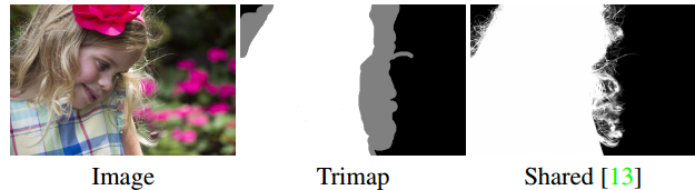
An example of matting - input data includes trimap.

The matting task is different from other image processing tasks, since the input data includes not only the image, but also trimap, the outline of the edges of the images, which makes matting the problem of "semi-controlled" learning.

We experimented a bit with matting using our segmentation as a trimap, but did not achieve significant results.

Another problem was the lack of dataset suitable for learning.

Results

As stated at the beginning, our goal was to create a meaningful product through deep learning. As you can see in Alon's posts, implementation is getting easier and faster. On the other hand, with the training model things are worse - training, especially when it is held overnight, requires careful planning, debugging and recording of results.

It is not easy to balance between research and attempts to do something new, as well as routine training and improvement. Since we use deep learning, we always have the feeling that a more advanced model is just around the corner, or just the model we need, and another Google search, or another read article will lead us to the desired. But in practice, our actual improvements were due to the fact that we “squeezed” more and more of our original model. And we still feel that we can squeeze so much more.

We had a lot of fun doing this work, which a few months ago seemed like science fiction.

greenScreen.AI