Random evolutionary strategies in machine learning

Neural networks do not study like people. Neural network optimization is actually a gradient descent over a certain loss function $$$E (\ theta)$ where variables are layer weights $$$\ theta$ . This is a very powerful approach to system tuning, which is also used in physics, economics and many other fields. At the moment, many specific gradient descent methods have been proposed, but they all suggest that the gradient $$$E (\ theta)$ behaves well: there are no cliffs, where it increases abruptly, or a plateau, where it vanishes. The first problem can be dealt with using the gradient clipping, but the second makes you think carefully. Piecewise linear or discrete function is nontrivially limited to more pleasant function.

• in many areas reinforcement learning (hereinafter RL)
• in VAE with discrete latent variables
• in GAN with discrete generators

What to do in such situations?

Under the cut there are many formulas and gifs.

About five years ago , articles began to appear that explored a different approach to learning: instead of smoothing the objective function, let’s take the gradient in such cases. In a certain way, sampling values $$$E (\ theta)$ , we can assume where to go, even if at the current point the derivative is exactly zero. Not that the sampling approaches were particularly new - Monte Carlo has been friends with neural networks for a long time - but recently new interesting results have been obtained.

The basis of this article was taken in the blog Ferenc Huszár.
')

Random Evolution Strategy (ES)

Let's start with the simplest approach, which regained its popularity after the OpenAI article in 2017. I note that evolutionary strategies do not have a very good name associated with the development of this family of algorithms. With genetic algorithms ES are connected very remotely - only by random change of parameters. It is much more productive to think about ES as a method for estimating the gradient using sampling. We sample from the normal distribution. $$$\ mathbb {N} (0, \ sigma)$ several perturbation vectors $$$\ epsilon$ , we take the expectation of the resulting values ​​of the objective function, and we assume that

$$

$$\ frac {\ delta} {\ delta \ theta} E (\ theta) \ approx \ frac {1} {\ sigma ^ 2} \ mathbb {E} _ {\ epsilon \ sim \ mathbb {N} (0, \ sigma)} [\ epsilon E (\ theta + \ epsilon)]$$

The idea is quite simple. With a standard gradient descent, at each step we look at the inclination of the surface on which we are located and move in the direction of the greatest gradient. In ES, we “fire” a nearby neighborhood with points where we can supposedly move, and move in the direction where most points with the greatest height difference fall (and the farther the point, the more weight is attached to it).


The proof is also simple. Suppose that in fact the loss function can be expanded into a Taylor series in $$$\ theta$ :

$$

$$E (\ theta + \ epsilon) = E (\ theta) + E '(\ theta) \ epsilon + \ frac {E' '(\ theta) \ epsilon ^ 2} {2} + O (\ epsilon ^ 3 )$$

Multiply both sides by $$$\ epsilon$ :

$$

$$E (\ theta + \ epsilon) \ epsilon = E (\ theta) \ epsilon + E '(\ theta) \ epsilon ^ 2 + \ frac {E' (\ theta) \ epsilon ^ 3} {2} + O (\ epsilon ^ 4)$$

Throw away $$$O (\ epsilon ^ 4)$ and take the expectation from both sides:

$$

$$\ mathbb {E} _ {\ epsilon \ sim \ mathbb {N} (0, \ sigma)} [E (\ theta + \ epsilon) \ epsilon] = \ mathbb {E} _ {\ epsilon \ sim \ mathbb {N} (0, \ sigma)} [E (\ theta) \ epsilon + E '(\ theta) \ epsilon ^ 2 + \ frac {E' '(\ theta) \ epsilon ^ 3} {2}]$$

But the normal distribution is symmetrical: $$$\ mathbb {E} _ {\ epsilon \ sim \ mathbb {N} (0, \ sigma)} [\ epsilon] = 0$ , $$$\ mathbb {E} _ {\ epsilon \ sim \ mathbb {N} (0, \ sigma)} [\ epsilon ^ 2] = \ sigma ^ 2$ , $$$\ mathbb {E} _ {\ epsilon \ sim \ mathbb {N} (0, \ sigma)} [\ epsilon ^ 3] = 0$ :

$$

$$\ mathbb {E} _ {\ epsilon \ sim \ mathbb {N} (0, \ sigma)} [E (\ theta + \ epsilon) \ epsilon] = E '(\ theta) \ sigma ^ 2$$

Divide by $$$\ sigma ^ 2$ and get the original statement.

In the case of a piecewise-step function, the resulting estimate $$$\ frac {\ delta} {\ delta \ theta} E (\ theta)$ will represent the gradient of the smoothed function without the need to calculate the specific values ​​of this function at each point; The article provides more rigorous statements. Also in the case when the loss function depends on discrete parameters $$$x$ (those. $$$E (\ theta) = \ mathbb {E} _ {x} E (\ theta, x)$ ), it can be shown that the estimate remains valid, since in the proof one can interchange the order of taking the expectation

$$

$$\ mathbb {E} _ {\ epsilon} \ epsilon E (\ theta + \ epsilon) = \ mathbb {E} _ {\ epsilon} \ epsilon \ mathbb {E} _ {x} E (\ theta + \ epsilon , x) = \ mathbb {E} _ {x} \ mathbb {E} _ {\ epsilon} \ epsilon E (\ theta + \ epsilon, x)$$

Which is often not possible for ordinary SGD.

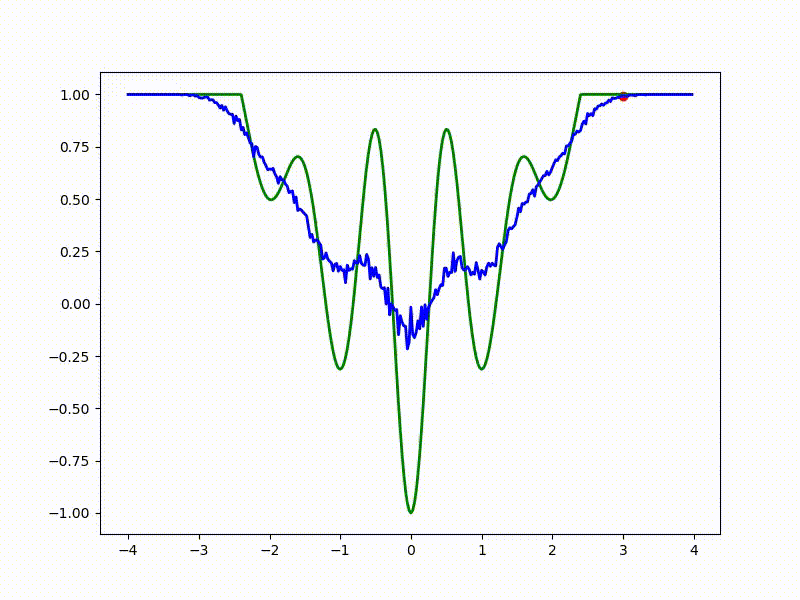
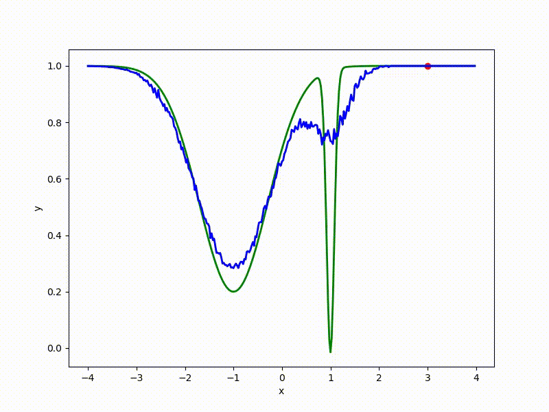
Let's look at the function smoothed by sampling from $$$\ mathbb {N} (0, \ sigma)$ . Once again: in fact, it makes no sense to count $$$E (\ theta)$ , we only need derivatives. However, such visualizations help to understand which landscape actually produces gradient descent. So, the green graph is the original function, blue is what it looks like for the optimization algorithm after evaluating the gradient by sampling:

$$$\ sigma = 0.35$ :

$$$\ sigma = 0.2$ :

$$$\ sigma = 0.1$ :

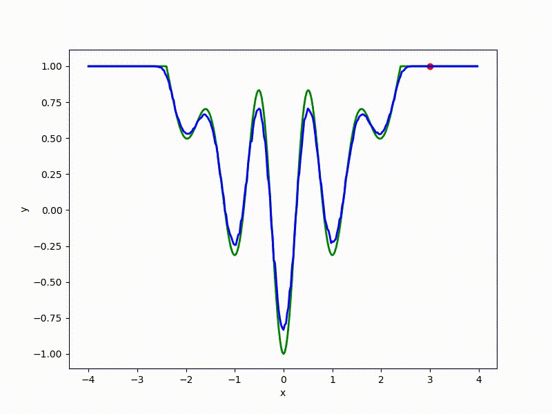
The greater the sigma distribution, the less the local structure of the function manifests itself. When the sampling algorithm is too large, the optimization algorithm does not show narrow minima and hollows, from which one can go from one good state to another. If it is too small, the gradient descent may never start if the initialization point was chosen unsuccessfully.

More charts:


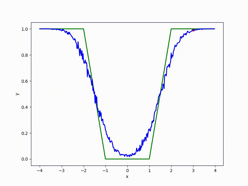
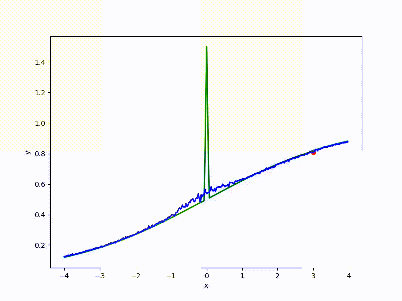
Gradient descent automatically finds the most stable minimum in the middle of the plateau and “tunnels” through a sharp peak.

The advantages of this approach compared with the usual gradient descent:

• As mentioned, $$$E (\ theta)$ not required to be differentiable. At the same time, no one forbids the use of ES, even when you can honestly calculate the gradient.
• ES is trivially parallel. Although there are parallel versions of SGD, they require weight transfer. $$$\ theta_i$ between nodes-workers or nodes and the central server. It is very expensive when there are many layers. In the case of evolutionary strategies, each workstation can read its own set $$$E_i = E (\ theta + \ epsilon_i)$ . Forward $$$E_i$ it's pretty simple - it's usually just scalars. $$$\ epsilon_i$ forwarding is as difficult as $$$\ theta$ however, there is no need to do this: if all the nodes know the algorithm for sampling random numbers and a seed generator, they can simulate $$$\ epsilon_i$ each other ! The performance of such a system increases almost linearly when scaled, which makes the distributed version of ES just incredibly fast when a large number of stations are available for training. OpenAI reports about learning MuJoCo in 10 minutes on 80 machines with 1440 CPUs.
• Sampling $$$\ theta$ makes noise in the gradient calculation, which makes learning more sustainable. Compare with dropout when learning neural networks in the usual way.
• ES does not depend on frame-skip with RL (see, for example, here ) - one less hyper parameter.
• It is also argued that evolutionary strategies allow learning more easily than regular SGD, when a large amount of time can pass between an action in RL and a positive response, and in noisy conditions, when it is not clear which change helped improve the result (less the situation when the network at the beginning of training for a long time can not understand what to do in a virtual environment and only jerks in place).

What are the disadvantages?

• The graphs in the OpenAI article do not look so radiant. Training with ES takes 2-10 times more epochs than training with TRPO. The authors are protected by the fact that when a large number of working machines are available, the real time spent is 20-60 times less (although each update brings less benefit, we can do them much more often). That's great, of course, but where else would you get 80 work nodes. Plus, as if the final results are a bit worse. Perhaps you can "finish" the network with a more accurate algorithm?
• Noise in gradients - a double edged sword. Even with one-dimensional optimization, they are slightly unstable (see the noise on the blue curves in the graphs above), what can we say when $$$\ theta$ very multidimensional. So far, it is not clear how serious the problem is, and what can be done about it, except for how to increase the size of the sampling sample.
• It is not known whether it is possible to effectively apply ES in regular training with a teacher. OpenAI honestly reports that on a regular MNIST ES it can be 1000 (!) Times slower than normal optimization.

ES variations

An additional positive quality of evolutionary strategies is that they only tell us how to calculate the derivative, and do not force us to rewrite the backpropagation algorithm for an error completely. Everything that can be applied to backprop-SGD can also be applied to ES: Nesterov's impulse, Adam-like algorithms, batch normalization. There are several specific additional techniques, but so far more research is needed, under what circumstances they work:

• ES allows to evaluate not only the first, but also the second derivative $$$E (\ theta)$ . To obtain a formula, it suffices to paint the Taylor series in the proof above to the fifth term, and not to the third and subtract the resulting formula from it for the first derivative. However, it seems that it is worth doing it only out of scientific curiosity, since the assessment turns out to be terribly unstable, and Adam already allows you to emulate the action of the second derivative in the algorithm.
• It is not necessary to use the normal distribution. Obvious applicants are the Laplace distribution and the t-distribution, but you can also come up with more exotic options.
• It is not necessary to sample only the current one. $$$\ theta$ . If you remember the history of movement in the parameter space, you can sample the weights around the point a bit in the direction of movement.
• During training, you can periodically jump not in the direction of the gradient but simply to the point with the smallest $$$E (\ theta + \ epsilon_i)$ . On the one hand, it destabilizes learning even more, on the other hand, this approach works well in highly non-linear cases with a large number of local minima and saddle points.
• The Uber article from December 2017 offers novelty reward seeking evolution strategies (NSR-ES): an additional member is added to the weights update formulas to encourage new behavioral strategies. The idea of ​​introducing diversity into reinforcement learning is not new, it is obvious that they will try to stick it here. The resulting learning algorithms give noticeably better results in some Atari dataset games.
• There is also an article stating that it is not necessary to send results from all nodes to all other nodes: a thinned graph of communication between workstations not only works faster, but also produces better results (!). Apparently, not communicating with all fellow students works as an additional regularization, like a dropout.

See also this article , which additionally reflects on the difference in behavior of ES and TRPO in different types of parameter landscapes, this article , describing in more detail the relationship between ES and SGD, this article proving the extraterrestrial origin of the Egyptian pyramids, and this article comparing ES from OpenAI with older classic es.

Variational optimization (VO)

Hmm, but why did not say a word about the change $$$\ sigma$ during training? It would be logical to reduce it, because the longer the training goes, the closer we are to the desired result, therefore you need to pay more attention to the local landscape $$$E (\ theta)$ . That's just exactly how to change the standard deviation? I do not want to invent some tricky scheme ...

It turns out that everything has already been invented! Evolution strategies are a special case of variation optimization for fixed $$$\ sigma$ .

Variational optimization is based on an auxiliary statement about the variational constraint from above: the global minimum of the function $$$E (\ theta)$ can not be more than the average value $$$E (\ theta_i)$ how would we these $$$\ theta_i$ nor sampled:

$$

$$\ min _ {\ theta} E (\ theta) \ leq \ min _ {\ eta} \ mathbb {E} _ {\ theta \ sim p (\ theta | \ eta)} [E (\ theta)] = \ min_ {\ eta} J (\ eta, E)$$

Where $$$J (\ eta, E)$ - variational functional, the global minimum of which coincides with the global minimum $$$E$ . Notice that now minimization does not go according to the initial parameters. $$$\ theta$ , and by the distribution parameters, from which we sampled these parameters - $$$\ eta$ . Also note that even if $$$E$ was non-differentiable $$$J$ differentiable if differentiable distribution $$$p (\ theta | \ eta)$ , and the derivative can be expressed as:

$$

$$\ frac {\ delta} {\ delta \ eta} \ mathbb {E} _ {\ theta \ sim p (\ theta | \ eta)} [E (\ theta)] = \ frac {\ delta} {\ delta \ eta} \ int p (\ theta | \ eta) E (\ theta) d \ theta$$

$$

$$= \ int \ frac {\ delta} {\ delta \ eta} p (\ theta | \ eta) E (\ theta) d \ theta$$

$$

$$= \ int p (\ theta | \ eta) E (\ theta) \ frac {\ delta} {\ delta \ eta} \ log {p (\ theta | \ eta)} d \ theta$$

$$

$$= \ mathbb {E} _ {\ theta \ sim p (\ theta | \ eta)} E (\ theta) \ frac {\ delta} {\ delta \ eta} \ log {p (\ theta | \ eta) }$$

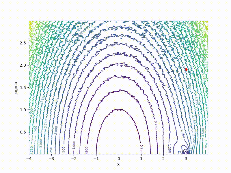
If a $$$p (\ theta | \ eta)$ - Gaussian distribution with a fixed dispersion, from this formula it is easy to obtain a formula for ES. But what if $$$\ sigma$ not fixed? Then for every weight in $$$\ theta$ we have two parameters in $$$\ eta$ : center and standard deviation of the corresponding Gaussian. The dimension of the task doubles! The easiest way to show on a one-dimensional example. Here is a top view of the resulting transformation landscape for the function from the previous section:

And descending through it:

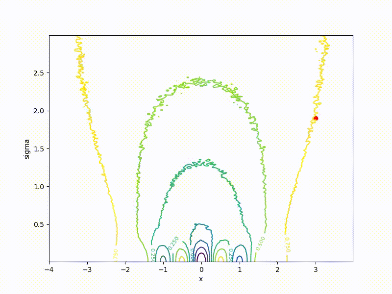
Its values ​​are at the point $$$(\ mu, \ sigma)$ correspond to the mean values ​​sampled from a point $$$\ mu = x$ using a normal distribution with standard deviation $$$\ sigma$ . Note that

• Again: in real life it makes no sense to consider counting this function. As in the case of ES, we need only a gradient.
• Now we minimize $$$(\ mu, \ sigma)$ , but not $$$x$ .
• The smaller $$$\ sigma$ the larger the cross section $$$J$ resembles the original function $$$E$
• Global minimum $$$J$ achieved at $$$\ mu = 0, \ sigma \ rightarrow 0$ . In the end, we only need $$$\ mu$ , but $$$\ sigma$ can be discarded.
• The global minimum of the one-dimensional function is quite difficult to get into - it is fenced with high walls. However, if you start from a point with a large $$$\ sigma$ , it becomes much easier to do this, since the greater the smoothing, the stronger the cross section of the function resembles the ordinary quadratic function.
• However, it is better to use Adam to get into a narrow hollow of a minimum.

What are the benefits of introducing variational optimization? It turns out that in ES there was a fixed $$$\ sigma$ his formula could lead us towards suboptimal minima: the more $$$\ sigma$ , the less on a landscape of the smoothed function, deep, but narrow minima are noticeable.

Since in VO $$$\ sigma$ Permenny, we have at least a chance to get into the real global minimum.

The disadvantages are obvious: even in the simplest case, the dimension of the problem is doubled, what can we say about the case when we want to have $$$\ sigma_i$ on every direction. Gradients are becoming even more unstable.

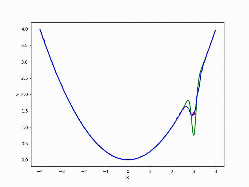
Recall the chart above with the “wall” in the middle. VO feels it even less:

(the former wall is a small thing from the bottom in the middle)

Although the convergence to the global minimum is not guaranteed even for simple cases, we are more likely to get at least somewhere with imperfect initialization:


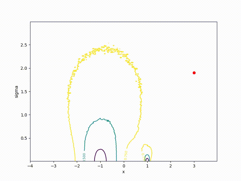
Or even get out of the bad spatial initialization section:

Conclusion

An article in OpenAI brought to the variational optimization a trick with a common seed of random number generators of various nodes. But so far (it seems?) There are no articles that evaluate the real acceleration from it. It seems to me, in the near future, we will see them. If they are encouraging, and if ES and VO are extended to training with a teacher, perhaps a paradigm shift in machine learning awaits us.

Download the code with which the visualization was built, you can here . Look at other visualizations and learn about the relationship of the above methods with genetic algorithms, Natural Evolution Strategies and Covariance-Matrix Adaptation Evolution Strategy (CMA-ES) here . Write in the comments if someone is interested to see how ES and VO will behave on a particular function. Thanks for attention!