Searchless method for calculating controller settings using Python

Introduction
The searchless method is a simple, reliable and universal method for calculating the settings of suboptimal regulators, including such algorithms as PD, Traffic Control and PIDD [1].
However, the software implementation of this method given in [1] has a number of drawbacks, which complicates its use in microprocessor-based control devices.
')
Among the shortcomings are the following:
Ambiguity in determining the operating frequency range, which, even with a smoothing link in the structure of the transfer function of the regulator, can lead to negative settings;
In [1], for the implementation of the searchless method of calculating regulators, the transfer function of an object of the form is considered:
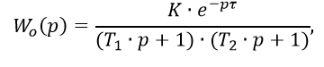
that with the second degree of the operator p in the denominator limits the accuracy of the dynamic identification of the control object [2].
Formulation of the problem:
1. By means of the high-level Python programming language, determine the maximum and minimum frequencies from the sub-optimal controller CFCs so that, at the maximum of the frequency, the imaginary and real parts of the transfer function are positive;
2. Using the scipy library. optimize the high-level programming language Python found by the transfer function of the suboptimal regulator regulator settings, and the library means scipy. integrate to obtain transient characteristics of a closed-loop control system;
3. For a more accurate identification of the object, use the transfer function in calculations, which has the third power of the operator p in the denominator;

4. Compare the transient characteristics of a closed system, obtained by search [3] and searchless methods;
5. Build the transient response for the PIDD algorithm using the searchless method, compare it by the integral quadratic control quality criterion with the PID algorithm.
Theory
Consider the block diagram of the single-loop control system:

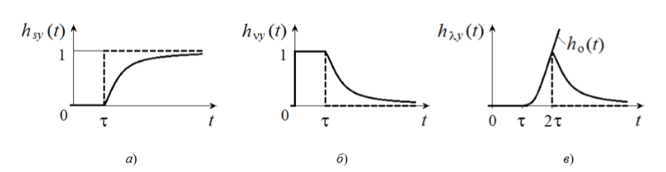
The algorithm of the optimal controller depends on the point of application of the step input. The following figure shows the transient characteristics of a closed system with respect to effects: a) ─ defining s (t); b) ─ external v (t); c) ─ internal λ (t):
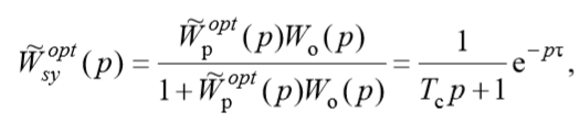
The optimal regulator after the time delay τ must fully reproduce the single action specified for the system input s (t) = 1. For this, the transfer function of a closed system must be equal to:

from the above equation we obtain the ratio for the transfer function of the optimal controller:
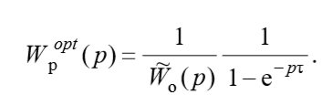 (one)
(one)In the complex-frequency characteristic (1) there are gaps with a period τ, which leads to a loss of stability of the system. Therefore, to obtain the transfer function of the suboptimal regulator, you need to apply smoothing using the simplest inertial element with the transfer function:
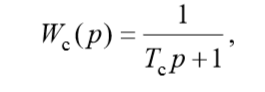
then the desired transfer function of the suboptimal closed-loop system can be represented as:
and the transfer function of the suboptimal regulator is
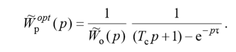 (2)
(2)Using the transfer function of a suboptimal regulator (2) may not give the desired transition process, since the structure of the suboptimal regulator depends on the structure of the transfer function of the object.
For example, when regulating the temperature of superheated steam, the object has an extreme transient response. In this case, as a smoothing one should choose an integrating differentiation (ID) link with the transfer function:
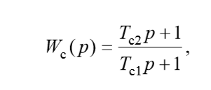
then the transfer function of the suboptimal regulator is written as:
 (3)
(3)Having the transfer functions of suboptimal regulators (2), (3), one can proceed to the consideration of the non-search method for determining settings.
Calculation of the optimal settings of linear regulators by the searchless method [1]:
Using the least squares approximation of the frequency characteristics of suboptimal (2) or (3) regulators, using the example of PIDD and PID regulators with four c1, c2, c3, c4 and three c1, c2, c3 parameters, respectively, will be performed.
Special cases of the PID regulator will be P, PI, PD and PDD laws of regulation. For the P controller, it is necessary to equate to 0 the settings, c2, c3, c4 for PI - c3, c4, for PD ―c2, c4 and for traffic regulations c2.
The linear frequency response of the PID controller will be represented as:
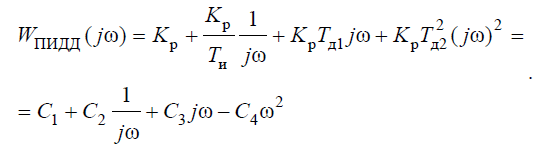 (four)
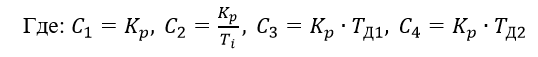
We write the sum of squared residuals for N vectors of frequency characteristics for all types of regulators

Implementing a non-search method using Python
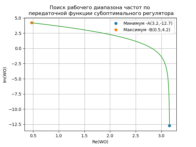
The definition of the maximum and minimum values of the operating frequency by the QFC of the suboptimal regulator:
# -*- coding: utf8 -*- import numpy as np from scipy.integrate import quad from scipy.optimize import * import matplotlib.pyplot as plt T1=14;T2=18;T3=28;T=15;K=0.9;tau=6.4# ( ) fmin=0.004# fmax=0.08# df=0.0001# n=np.arange(fmin,fmax,df)# def W(w):# j=(-1)**0.5 return ((K*(np.exp(-tau*j*w))/((T1*j*w+1)*(T2*j*w+1)*(T3*j*w+1)))) def WO(w):# j=(-1)**0.5 return (1/(K*(T*j*w+1-np.exp(-tau*j*w))/((T1*j*w+1)*(T2*j*w+1)*(T3*j*w+1)))) def ReWO(w):# j=(-1)**0.5 return WO(w).real def ImWO(w):# j=(-1)**0.5 return WO(w).imag S1=[ReWO(w) for w in n] S2=[ImWO(w) for w in n] plt.title(" \n ") plt.xlabel("Re(WO)") plt.ylabel("Im(WO)") plt.plot(ReWO(min(n)),ImWO(min(n)),'o',label=' -(%s,%s)'%(round(ReWO(min(n)),1),round(ImWO(min(n)),1))) plt.plot(ReWO(max(n)),ImWO(max(n)),'o',label=' -B(%s,%s)'%(round(ReWO(max(n)),1),round(ImWO(max(n)),1))) plt.plot(S1,S2) plt.grid(True) plt.legend(loc='best') plt.show() After finding with the help of the variables fmin, fmax, df of the required QFC, we obtain
Comparative analysis of search and searchless methods on the example of the PID controller and the transfer function of the object with the third degree of the operator p in the denominator:
For a comparative analysis of the search-and-search method, we use the results of the search method in my publication [3] for the parameters of the object T1 = 14; T2 = 18; T3 = 28; K = 0.9; tau = 6.4, which were used in solving the first problem.
Search method listing [3]
# -*- coding: utf8 -*- import numpy as np from scipy.integrate import quad from scipy.optimize import * import matplotlib.pyplot as plt import matplotlib as mpl mpl.rcParams['font.family'] = 'fantasy' mpl.rcParams['font.fantasy'] = 'Comic Sans MS, Arial' T1=14;T2=18;T3=28;K=0.9;tau=6.4# , , m=0.366;m1=0.221# n= np.arange(0.001,0.15,0.0002)# Kr-Ki n1=np.arange(0.00001,0.12,0.0001)# Ki=f(w) n2=np.arange(0.0002,0.4,0.0001)# def WO(m,w):# j=(-1)**0.5 return K*np.exp(-tau*(-m+j)*w)/((T1*(-m+j)*w+1)*(T2*(-m+j)*w+1)*(T3*(-m+j)*w+1)) def WR(w,Kr,Ti,Td):# j=(-1)**0.5 return Kr*(1+1/(j*w*Ti)+j*w*Td) def ReW(m,w):# j=(-1)**0.5 return WO(m,w).real def ImW(m,w):# j=(-1)**0.5 return WO(m,w).imag def A0(m,w):# return -(ImW(m,w)*m/(w+w*m**2)+ReW(m,w)/(w+w*m**2)) def Ti(alfa,m,w):# return (-ImW(m,w)-(ImW(m,w)**2-4*((ReW(m,w)*alfa*w-ImW(m,w)*alfa*w*m)*A0(m,w)))**0.5)/(2*(ReW(m,w)*alfa*w-ImW(m,w)*alfa*w*m)) def Ki(alfa,m,w):# return 1/(w*Ti(alfa,m,w)**2*alfa*(m*ReW(m,w)+ImW(m,w))-Ti(alfa,m,w)*ReW(m,w)+(m*ReW(m,w)-ImW(m,w))/(w+w*m**2)) def Kr(alfa,m,w):# if Ki(alfa,m,w)*Ti(alfa,m,w)<0: z=0 else: z=Ki(alfa,m,w)*Ti(alfa,m,w) return z def Kd(alfa,m,w):# return alfa*Kr(alfa,m,w)*Ti(alfa,m,w) alfa=0.2 Ki_1=[Ki(alfa,m1,w) for w in n] Kr_1=[Kr(alfa,m1,w) for w in n] Ki_2=[Ki(alfa,m,w) for w in n] Kr_2=[Kr(alfa,m,w) for w in n] Ki_3=[Ki(alfa,0,w) for w in n] Kr_3=[Kr(alfa,0,w) for w in n] plt.figure() plt.title(" \n alfa=%s"%alfa) plt.axis([0.0, round(max(Kr_3),4), 0.0, round(max(Ki_3),4)]) plt.plot(Kr_1, Ki_1, label=' m=%s'%m1) plt.plot(Kr_2, Ki_2, label=' m=%s'%m) plt.plot(Kr_3, Ki_3, label=' m=0') plt.xlabel(" - Ki") plt.ylabel(" - Kr") plt.legend(loc='best') plt.grid(True) alfa=0.7 Ki_1=[Ki(alfa,0.221,w) for w in n] Kr_1=[Kr(alfa,0.221,w) for w in n] Ki_2=[Ki(alfa,0.366,w) for w in n] Kr_2=[Kr(alfa,0.366,w) for w in n] Ki_3=[Ki(alfa,0,w) for w in n] Kr_3=[Kr(alfa,0,w) for w in n] plt.figure() plt.axis([0.0, round(max(Kr_3),3), 0.0, round(max(Ki_3),3)]) plt.title(" \n alfa=%s"%alfa) plt.plot(Kr_1, Ki_1, label=' m=%s'%m1) plt.plot(Kr_2, Ki_2, label=' m=%s'%m) plt.plot(Kr_3, Ki_3, label=' m=0') plt.xlabel(" - Ki") plt.ylabel(" - Kr") plt.legend(loc='best') plt.grid(True) alfa=1.2 Ki_1=[Ki(alfa,0.221,w) for w in n] Kr_1=[Kr(alfa,0.221,w) for w in n] Ki_2=[Ki(alfa,0.366,w) for w in n] Kr_2=[Kr(alfa,0.366,w) for w in n] Ki_3=[Ki(alfa,0,w) for w in n] Kr_3=[Kr(alfa,0,w) for w in n] plt.figure() plt.title(" \n alfa=%s"%alfa) plt.axis([0.0, round(max(Kr_3),3), 0.0, round(max(Ki_3),3)]) plt.plot(Kr_1, Ki_1, label=' m=%s'%m1) plt.plot(Kr_2, Ki_2, label=' m=%s'%m) plt.plot(Kr_3, Ki_3, label=' m=0') plt.xlabel(" - Ki") plt.ylabel(" - Kr") plt.legend(loc='best') plt.grid(True) plt.figure() plt.title(" \n m=%s"%m) alfa=0.2 Ki_2=[Ki(alfa,m,w) for w in n] Kr_2=[Kr(alfa,m,w) for w in n] plt.plot(Kr_2, Ki_2,label=' allfa=Td/Ti =%s'%alfa) alfa=0.4 Ki_2=[Ki(alfa,m,w) for w in n] Kr_2=[Kr(alfa,m,w) for w in n] plt.plot(Kr_2, Ki_2,label=' allfa=Td/Ti =%s'%alfa) alfa=0.7 Ki_2=[Ki(alfa,m,w) for w in n] Kr_2=[Kr(alfa,m,w) for w in n] plt.plot(Kr_2, Ki_2,label=' allfa=Td/Ti =%s'%alfa) alfa=1.2 Ki_2=[Ki(alfa,m,w) for w in n] Kr_2=[Kr(alfa,m,w) for w in n] plt.plot(Kr_2, Ki_2,label=' allfa=Td/Ti =%s'%alfa) plt.axis([0.0, round(max(Kr_2),3), 0.0, round(max(Ki_2),3)]) plt.legend(loc='best') plt.grid(True) plt.figure() plt.title(" Ki=f(w)") Ki_1=[Ki(0.2,m,w) for w in n1] Ki_2=[Ki(0.7,m,w) for w in n1] Ky=max([round(max(Ki_1),4),round(max(Ki_2),4)]) plt.axis([0.0,round(max(n1),4),0.0, Ky]) plt.plot(n1, Ki_1,label='allfa=Td/Ti =0.2, m=0.366') plt.plot(n1, Ki_2,label='allfa=Td/Ti =0.7, m=0.366') plt.legend(loc='best') plt.grid(True) maxKi=max( [Ki(0.7,m,w) for w in n1]) wa=round([w for w in n1 if Ki(0.7,m,w)==maxKi][0],3) Ki1=round(Ki(0.7,m,wa),3) Kr1=round(Kr(0.7,m,wa),3) Ti1=round(Kr1/Ki1,3) Td1=round(0.7*Ti1,3) d={} d[0]= " №1 (wa =%s,m=0.366,alfa=0.7): Kr=%s; Ti=%s; Ki=%s; Td=%s "%(wa,Kr1,Ti1,Ki1,Td1) print(d[0]) maxKi=max( [Ki(0.2,m,w) for w in n1]) wa=round([w for w in n1 if Ki(0.2,m,w)==maxKi][0],3) Ki2=round(Ki(0.2,m,wa),3) Kr2=round(Kr(0.2,m,wa),3) Ti2=round(Kr2/Ki2,3) Td2=round(0.2*Ti2,3) d[1]= " №2 (wa =%s,m=0.366,alfa=0.2): Kr=%s; Ti=%s; Ki=%s; Td=%s "%(wa,Kr2,Ti2,Ki2,Td2) print(d[1]) wa=fsolve(lambda w:Ki(0.7,m,w)-0.14,0.07)[0] wa=round(wa,3) Ki3=round(Ki(0.7,m,wa),3) Kr3=round(Kr(0.7,m,wa),3) Ti3=round(Kr3/Ki3,3) Td3=round(0.7*Ti3,3) d[2]= " №3 (wa =%s,m=0.366,alfa=0.7): Kr=%s; Ti=%s; Ki=%s; Td=%s "%(wa,Kr3,Ti3,Ki3,Td3) print(d[2]) def Wsys(w,Kr,Ti,Td): j=(-1)**0.5 return (WO(0,w)*WR(w,Kr,Ti,Td)/(1+WO(0,w)*WR(w,Kr,Ti,Td))) Wsys_1=[abs(Wsys(w,Kr1,Ti1,Td1)) for w in n2] Wsys_2=[abs(Wsys(w,Kr2,Ti2,Td2)) for w in n2] Wsys_3=[abs(Wsys(w,Kr3,Ti3,Td3)) for w in n2] plt.figure() plt.title("- \n ") plt.plot(n2, Wsys_1,label=' №1 ') plt.plot(n2, Wsys_2,label=' №2 ') plt.plot(n2, Wsys_3,label=' №3 ') plt.legend(loc='best') plt.grid(True) def ReWsys(w,t,Kr,Ti,Td): return(2/np.pi)* (WO(0,w)*WR(w,Kr,Ti,Td)/(1+WO(0,w)*WR(w,Kr,Ti,Td))).real*(np.sin(w*t)/w) def h(t,Kr,Ti,Td): return quad(lambda w: ReWsys(w,t,Kr,Ti,Td),0,0.6)[0] tt=np.arange(0,300,3) h1=[h(t,Kr1,Ti1,Td1) for t in tt] h2=[h(t,Kr2,Ti2,Td2) for t in tt] h3=[h(t,Kr3,Ti3,Td3) for t in tt] I1=round(quad(lambda t: h(t,Kr1,Ti1,Td1), 0,200)[0],3) I11=round(quad(lambda t: h(t,Kr1,Ti1,Td1)**2,0, 200)[0],3) I2=round(quad(lambda t: h(t,Kr2,Ti2,Td2), 0,200)[0],3) I21=round(quad(lambda t: h(t,Kr2,Ti2,Td2)**2,0, 200)[0],3) I3=round(quad(lambda t: h(t,Kr3,Ti3,Td3), 0,200)[0],3) I31=round(quad(lambda t: h(t,Kr3,Ti3,Td3)**2,0, 200)[0],3) print(" I1 =%s ( №1)"%I1) print(" I2 =%s ( №1"%I11) print(" I1 =%s ( №2 )"%I2) print(" I2 =%s ( №2)"%I21) print(" I1 =%s ( №3 )"%I3) print(" I2 =%s ( №3)"%I31) Rez=[I1+I11,I2+I21,I3+I31] In=Rez.index(min(Rez)) print(" :\n %s"%d[In]) plt.figure() plt.title(" \n ") plt.plot(tt,h1,'r',linewidth=1,label=' №1 ') plt.plot(tt,h2,'b',linewidth=1,label=' №2 ') plt.plot(tt,h3,'g',linewidth=1,label=' №3 ') plt.legend(loc='best') plt.grid(True) plt.show() Text output results:
Settings No. 1 of the PID controller (wa = 0.066, m = 0.366, alfa = 0.7): Kr = 4.77; Ti = 21,682; Ki = 0.22; Td = 15.177
Settings # 2 of the PID controller (wa = 0.056, m = 0.366, alfa = 0.2): Kr = 2.747; Ti = 50.87; Ki = 0.054; Td = 10.174
Settings No. 3 of the PID controller (wa = 0.085, m = 0.366, alfa = 0.7): Kr = 3.747; Ti = 26.387; Ki = 0.142; Td = 18.471
Linear integral quality criterion I1 = 194.65 (settings №1)
Quadratic integral quality criterion I2 = 222.428 (settings №1
Linear integral quality criterion I1 = 179.647 (setting No. 2)
The quadratic integral quality criterion I2 = 183.35 (settings №2)
Linear integral quality criterion I1 = 191.911 (setting number 3)
Quadratic integral quality criterion I2 = 204.766 (setting No. 3)
Optimal parameters by integral criteria:
Settings # 2 of the PID controller (wa = 0.056, m = 0.366, alfa = 0.2): Kr = 2.747; Ti = 50.87; Ki = 0.054; Td = 10.174
Program listing for comparing regulator settings calculation methods
# -*- coding: utf8 -*- import numpy as np from scipy.integrate import quad from scipy.optimize import * import matplotlib.pyplot as plt T1=14;T2=18;T3=28;T=15;K=0.9;tau=6.4# T fmin=0.004 fmax=0.08 df=0.0001 n=np.arange(fmin,fmax,df) def W(w):# j=(-1)**0.5 return ((K*(np.exp(-tau*j*w))/((T1*j*w+1)*(T2*j*w+1)*(T3*j*w+1)))) def WO(w):# j=(-1)**0.5 return (1/(K*(T*j*w+1-np.exp(-tau*j*w))/((T1*j*w+1)*(T2*j*w+1)*(T3*j*w+1)))) def WR(w,c1,c2,c3):# j=(-1)**0.5 return (c1+c2/(j*w)+c3*j*w) def NF(c1,c2,c3):# return sum([((WO(w)).real-WR(w,c1,c2,c3).real)**2+((WO(w)).imag-WR(w,c1,c2,c3).imag)**2 for w in n]) def fun2(x): return NF(*x) x0=[1,1,1] res = minimize(fun2, x0) time=np.arange(0,300,1) e1=round(res['x'][0],3) e2=round(res['x'][1],3) e3=round(res['x'][2],3) Kp=round(res['x'][0],3) Ti=round((res['x'][0]/res['x'][1]),3) Ki=round((res['x'][0]/Ti),3) Td=round((res['x'][2]/res['x'][0]),3) print (" :",round(res['fun'],3)) print(" : Kp=%s; Ti=%s; Ki=%s; Td=%s "%(Kp,Ti,Ki,Td)) def h(t,e1,e2,e3): return quad(lambda w:(2/np.pi)*(((W(w))*WR(w,e1,e2,e3))/(1+(W(w))*WR(w,e1,e2,e3))).real*(np.sin(w*t)/w),0,max(n))[0] h1=[h(t,e1,e2,e3) for t in time] I1=round(quad(lambda t:h(t,e1,e2,e3), 0,300)[0],3)+round(quad(lambda t: h(t,e1,e2,e3)**2,0, 300)[0],3) Kp=2.747 Ti=50.87 Td=10.174 Ki=round(Kp/Ti,3) print(" : Kp=%s; Ti=%s; Ki=%s; Td=%s "%(Kp,Ti,Ki,Td)) e1=Kp e2=Kp/Ti e3=Td*Kp print (" [3]:",round(NF(e1,e2,e3),3)) h2=[h(t,e1,e2,e3) for t in time] I2=round(quad(lambda t:h(t,e1,e2,e3), 0,300)[0],3)+round(quad(lambda t: h(t,e1,e2,e3)**2,0, 300)[0],3) plt.title(" ( ) \n ") plt.plot(time,h1,'b',linewidth=2,label=' - %s ( )'%I1) plt.plot(time,h2,'g',linewidth=2,label=' - %s ( )'%I2) plt.legend(loc='best') plt.grid(True) plt.show() We get:
The estimated value of the objective function for the searchless method: 484.254
PID controller settings for the non-search method: Kp = 2.22; Ti = 42.904; Ki = 0.052; Td = 27.637
PID controller settings for the search method: Kp = 2.747; Ti = 50.87; Ki = 0.054; Td = 10.174
The calculated value of the objective function for the search method [3]: 2723.341
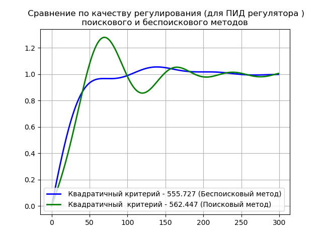
Obviously, the searchless method is easier to implement and provides better quality regulation.
Calculation of settings and obtaining the transient response of a closed system for a non-standard PIDD control algorithm:
# -*- coding: utf8 -*- import numpy as np from scipy.integrate import quad from scipy.optimize import * import matplotlib.pyplot as plt T1=14;T2=18;T3=28;T=15;K=0.9;tau=6.4 fmin=0.004 fmax=0.08 df=0.0001 n=np.arange(fmin,fmax,df) def W(w):# j=(-1)**0.5 return ((K*(np.exp(-tau*j*w))/((T1*j*w+1)*(T2*j*w+1)*(T3*j*w+1)))) def WO(w):# j=(-1)**0.5 return (1/(K*(T*j*w+1-np.exp(-tau*j*w))/((T1*j*w+1)*(T2*j*w+1)*(T3*j*w+1)))) def WR(w,c1,c2,c3,c4):# j=(-1)**0.5 return (c1+c2/(j*w)+c3*j*w-c4*w**2) def NF(c1,c2,c3,c4): return sum([((WO(w)).real-WR(w,c1,c2,c3,c4).real)**2+((WO(w)).imag-WR(w,c1,c2,c3,c4).imag)**2 for w in n]) def fun2(x): return NF(*x) x0=[1,1,1,1] res = minimize(fun2, x0) time=np.arange(0,300,1) e1=round(res['x'][0],3) e2=round(res['x'][1],3) e3=round(res['x'][2],3) e4=round(res['x'][3],3) print (" :",round(res['fun'],3)) def h(t,e1,e2,e3,c4): return quad(lambda w:(2/np.pi)*(((W(w))*WR(w,e1,e2,e3,e4))/(1+(W(w))*WR(w,e1,e2,e3,e4))).real*(np.sin(w*t)/w),0,max(n))[0] h1=[h(t,e1,e2,e3,e4) for t in time] I1=round(quad(lambda t:h(t,e1,e2,e3,e4), 0,300)[0],3)+round(quad(lambda t: h(t,e1,e2,e3,e4)**2,0, 300)[0],3) plt.title(" ") plt.plot(time,h1,'r',linewidth=2,label=' - %s'%I1) plt.legend(loc='best') plt.grid(True) plt.show() We get:
The estimated value of the objective function for the searchless method: 0.326
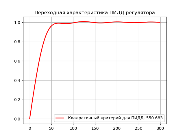
As one would expect, the PID algorithm provides the best quality of regulation than the PID, while it has the maximum approximation to the suboptimal regulator.
The program listings listed can be easily rebuilt to the regulators P, PI, PD and PDD regulatory laws. For the P controller, it is necessary to equate to 0 the settings, c2, c3, c4 for PI - c3, c4, for PD ―c2, c4 and for traffic regulations c2.
Findings:
The advantage of implementing the searchless method for calculating the settings of the regulators on the minimum of a quadratic criterion is considered
References:
1. The searchless method of calculating the settings of regulators on the minimum of a quadratic criterion
2. Dynamic identification of control objects.
3. Optimization of the PID controller settings according to the integral criterion of the quality of regulation.
Source: https://habr.com/ru/post/350030/
All Articles