Optimization of the PID controller settings by the integral criterion for the quality of regulation
Setting the task of assessing regulatory quality
Integral assessment of the quality of regulation characterizes the total deviation of the real transition process in the system from the idealized transition process.
As an idealized process, a stepwise (jump-like) transient process or an exponential process with specified exponent parameters is usually taken.
')
Until now, it remains unclear which of the integral criteria to choose linear or quadratic to optimize the settings of the regulators.
In this publication, the determination of the optimal controller settings is carried out on the basis of the optimality criterion as a sum of linear and quadratic integral indicators of the quality of regulation.
In order to make such a choice, it is first necessary to conduct a series of preliminary calculations for different values of the ratio of the time constants of differentiation and integration α = Td / Ti and choose several values of α, which provide the largest value of the ratio Kr / Ki.
After that, having several options for regulator settings, construct transients for them in a closed system and select the optimal settings according to the proposed criterion.
Software implementation of the calculation of the optimal controller settings
The calculation can be performed both in a mathematical package and in any programming language. However, due to the presence of powerful libraries for numerical integration and a simple implementation of searching local extrema in lists, I chose a high-level programming language Python.
To simplify the search procedures at the beginning of the program, it is advisable to establish the source data and provide ready-made frequency lists for each problem to be solved separately:
Preparation of source data
# -*- coding: utf8 -*- import numpy as np # from scipy.integrate import quad # import matplotlib.pyplot as plt # T1=14; T2=18; T3=28; K=0.9; tau=6.4# , , m=0.366; m1=0.221# n= np.arange(0.001,0.15,0.0002)# Kr-Ki n1=np.arange(0.00001,0.12,0.0001) # Ki=f(w) n2=np.arange(0.0002,0.4,0.0001) # We introduce the transfer function for the water heat exchanger taking into account the root index of oscillation m and the transfer function of the PID controller taking into account Kr, Ti, Td, the remaining functions are auxiliary:
Input of main and auxiliary functions with regard to complex arithmetic
def WO(m,w):# j=(-1)**0.5 return K*np.exp(-tau*(-m+j)*w)/((T1*(-m+j)*w+1)*(T2*(-m+j)*w+1)*(T3*(-m+j)*w+1)) def WR(w,Kr,Ti,Td):# j=(-1)**0.5 return Kr*(1+1/(j*w*Ti)+j*w*Td) def ReW(m,w):# j=(-1)**0.5 return WO(m,w).real def ImW(m,w):# j=(-1)**0.5 return WO(m,w).imag def A0(m,w):# return -(ImW(m,w)*m/(w+w*m**2)+ReW(m,w)/(w+w*m**2)) def Ti(alfa,m,w):# return (-ImW(m,w)-(ImW(m,w)**2-4*((ReW(m,w)*alfa*w-ImW(m,w)*alfa*w*m)*A0(m,w)))**0.5)/(2*(ReW(m,w)*alfa*w-ImW(m,w)*alfa*w*m)) def Ki(alfa,m,w):# return 1/(w*Ti(alfa,m,w)**2*alfa*(m*ReW(m,w)+ImW(m,w))-Ti(alfa,m,w)*ReW(m,w)+(m*ReW(m,w)-ImW(m,w))/(w+w*m**2)) def Kr(alfa,m,w):# if Ki(alfa,m,w)*Ti(alfa,m,w)<0: z=0 else: z=Ki(alfa,m,w)*Ti(alfa,m,w) return z def Kd(alfa,m,w):# return alfa*Kr(alfa,m,w)*Ti(alfa,m,w) Construct three planes for tuning the PID controller for the relations alfa = Td / Ti = 0.2, alfa = Td / Ti = 0.7 alfa = Td / Ti = 1.2.
Search for optimal alfa values
alfa=0.2 Ki_1=[Ki(alfa,m1,w) for w in n] Kr_1=[Kr(alfa,m1,w) for w in n] Ki_2=[Ki(alfa,m,w) for w in n] Kr_2=[Kr(alfa,m,w) for w in n] Ki_3=[Ki(alfa,0,w) for w in n] Kr_3=[Kr(alfa,0,w) for w in n] plt.figure() plt.title(" \n alfa=%s"%alfa) plt.axis([0.0, round(max(Kr_3),4), 0.0, round(max(Ki_3),4)]) plt.plot(Kr_1, Ki_1, label=' m=%s'%m1) plt.plot(Kr_2, Ki_2, label=' m=%s'%m) plt.plot(Kr_3, Ki_3, label=' m=0') plt.xlabel(" - Ki") plt.ylabel(" - Kr") plt.legend(loc='best') plt.grid(True) alfa=0.7 Ki_1=[Ki(alfa,0.221,w) for w in n] Kr_1=[Kr(alfa,0.221,w) for w in n] Ki_2=[Ki(alfa,0.366,w) for w in n] Kr_2=[Kr(alfa,0.366,w) for w in n] Ki_3=[Ki(alfa,0,w) for w in n] Kr_3=[Kr(alfa,0,w) for w in n] plt.figure() plt.axis([0.0, round(max(Kr_3),3), 0.0, round(max(Ki_3),3)]) plt.title(" \n alfa=%s"%alfa) plt.plot(Kr_1, Ki_1, label=' m=%s'%m1) plt.plot(Kr_2, Ki_2, label=' m=%s'%m) plt.plot(Kr_3, Ki_3, label=' m=0') plt.xlabel(" - Ki") plt.ylabel(" - Kr") plt.legend(loc='best') plt.grid(True) alfa=1.2 Ki_1=[Ki(alfa,0.221,w) for w in n] Kr_1=[Kr(alfa,0.221,w) for w in n] Ki_2=[Ki(alfa,0.366,w) for w in n] Kr_2=[Kr(alfa,0.366,w) for w in n] Ki_3=[Ki(alfa,0,w) for w in n] Kr_3=[Kr(alfa,0,w) for w in n] plt.figure() plt.title(" \n alfa=%s"%alfa) plt.axis([0.0, round(max(Kr_3),3), 0.0, round(max(Ki_3),3)]) plt.plot(Kr_1, Ki_1, label=' m=%s'%m1) plt.plot(Kr_2, Ki_2, label=' m=%s'%m) plt.plot(Kr_3, Ki_3, label=' m=0') plt.xlabel(" - Ki") plt.ylabel(" - Kr") plt.legend(loc='best') plt.grid(True) plt.figure( )For the stability margin m = 0.386 with values of alfa -0.2,0,4,0.7, we construct D-partitions to determine the critical values of alfa.
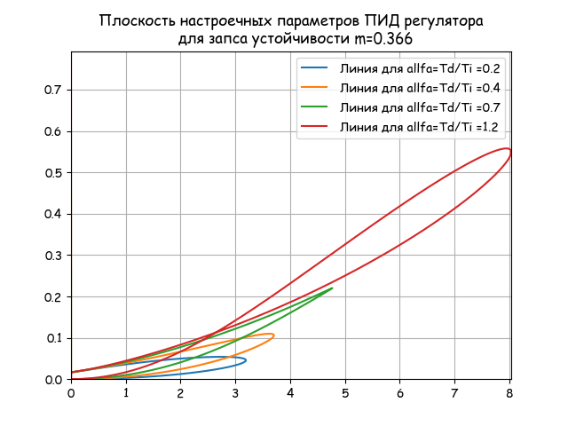
The total plane of all tuning parameters
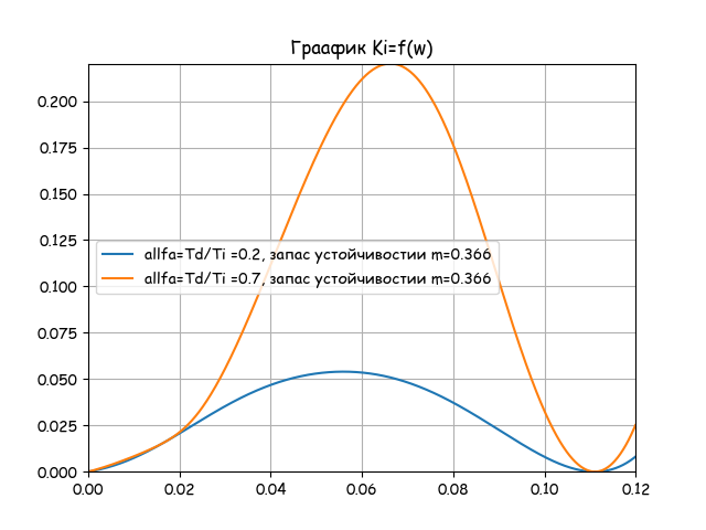
plt.title(" \n m=%s"%m) alfa=0.2 Ki_2=[Ki(alfa,m,w) for w in n] Kr_2=[Kr(alfa,m,w) for w in n] plt.plot(Kr_2, Ki_2,label=' allfa=Td/Ti =%s'%alfa) alfa=0.4 Ki_2=[Ki(alfa,m,w) for w in n] Kr_2=[Kr(alfa,m,w) for w in n] plt.plot(Kr_2, Ki_2,label=' allfa=Td/Ti =%s'%alfa) alfa=0.7 Ki_2=[Ki(alfa,m,w) for w in n] Kr_2=[Kr(alfa,m,w) for w in n] plt.plot(Kr_2, Ki_2,label=' allfa=Td/Ti =%s'%alfa) alfa=1.2 Ki_2=[Ki(alfa,m,w) for w in n] Kr_2=[Kr(alfa,m,w) for w in n] plt.plot(Kr_2, Ki_2,label=' allfa=Td/Ti =%s'%alfa) plt.axis([0.0, round(max(Kr_2),3), 0.0, round(max(Ki_2),3)]) plt.legend(loc='best') plt.grid(True) Build a graph of Ki versus frequency w for two alfa values detected from the previous graph: 0.2; 0.7 Ki settings are determined by resonant frequencies.
plt.figure() plt.title(" Ki=f(w)") Ki_1=[Ki(0.2,m,w) for w in n1] Ki_2=[Ki(0.7,m,w) for w in n1] Ky=max([round(max(Ki_1),4),round(max(Ki_2),4)]) plt.axis([0.0,round(max(n1),4),0.0, Ky]) plt.plot(n1, Ki_1,label='allfa=Td/Ti =0.2, m=0.366') plt.plot(n1, Ki_2,label='allfa=Td/Ti =0.7, m=0.366') plt.legend(loc='best') plt.grid(True) We define three options for setting the PID controller:
Obtaining the numerical values of the settings to select the optimal according to the proposed criterion
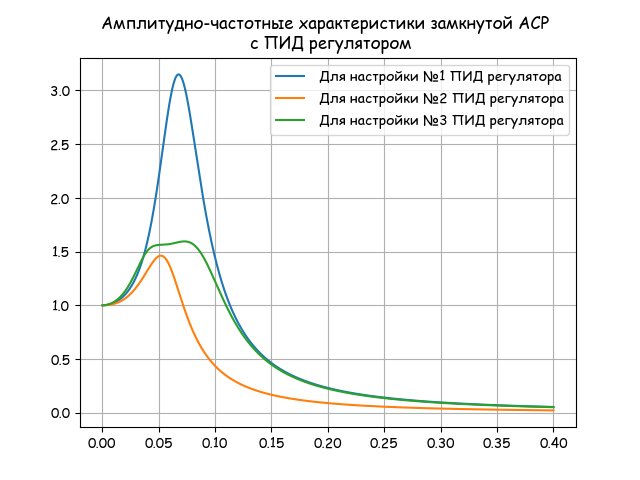
maxKi=max( [Ki(0.7,m,w) for w in n1]) wa=round([w for w in n1 if Ki(0.7,m,w)==maxKi][0],3) Ki1=round(Ki(0.7,m,wa),3) Kr1=round(Kr(0.7,m,wa),3) Ti1=round(Kr1/Ki1,3) Td1=round(0.7*Ti1,3) d=[] d[0]= " №1 (wa =%s,m=0.366,alfa=0.7): Kr=%s; Ti=%s; Ki=%s; Td=%s "%(wa,Kr1,Ti1,Ki1,Td1) print(d[0]) maxKi=max( [Ki(0.2,m,w) for w in n1]) wa=round([w for w in n1 if Ki(0.2,m,w)==maxKi][0],3) Ki2=round(Ki(0.2,m,wa),3) Kr2=round(Kr(0.2,m,wa),3) Ti2=round(Kr2/Ki2,3) Td2=round(0.2*Ti2,3) d[1]= " №2 (wa =%s,m=0.366,alfa=0.2): Kr=%s; Ti=%s; Ki=%s; Td=%s "%(wa,Kr2,Ti2,Ki2,Td2) print(d[1]) wa=fsolve(lambda w:Ki(0.7,m,w)-0.14,0.07)[0] wa=round(wa,3) Ki3=round(Ki(0.7,m,wa),3) Kr3=round(Kr(0.7,m,wa),3) Ti3=round(Kr3/Ki3,3) Td3=round(0.7*Ti3,3) d[2]= (" №3 (wa =%s,m=0.366,alfa=0.7): Kr=%s; Ti=%s; Ki=%s; Td=%s "%(wa,Kr3,Ti3,Ki3,Td3) print(d[2]) def Wsys(w,Kr,Ti,Td): j=(-1)**0.5 return (WO(0,w)*WR(w,Kr,Ti,Td)/(1+WO(0,w)*WR(w,Kr,Ti,Td))) Wsys_1=[abs(Wsys(w,Kr1,Ti1,Td1)) for w in n2] Wsys_2=[abs(Wsys(w,Kr2,Ti2,Td2)) for w in n2] Wsys_3=[abs(Wsys(w,Kr3,Ti3,Td3)) for w in n2] plt.figure() Determine the dynamics of ASR by the value of the frequency index of oscillation:
plt.title("- \n ") plt.plot(n2, Wsys_1,label=' №1 ') plt.plot(n2, Wsys_2,label=' №2 ') plt.plot(n2, Wsys_3,label=' №3 ') plt.legend(loc='best') plt.grid(True) We determine the optimal controller settings by the proposed integral criterion for the quality of regulation:

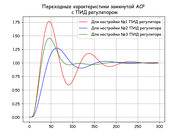
Numerical and graphical analysis of the optimal settings obtained
def ReWsys(w,t,Kr,Ti,Td): return(2/np.pi)* (WO(0,w)*WR(w,Kr,Ti,Td)/(1+WO(0,w)*WR(w,Kr,Ti,Td))).real*(np.sin(w*t)/w) def h(t,Kr,Ti,Td): return quad(lambda w: ReWsys(w,t,Kr,Ti,Td),0,0.6)[0] tt=np.arange(0,300,3) h1=[h(t,Kr1,Ti1,Td1) for t in tt] h2=[h(t,Kr2,Ti2,Td2) for t in tt] h3=[h(t,Kr3,Ti3,Td3) for t in tt] I1=round(quad(lambda t: h(t,Kr1,Ti1,Td1), 0,200)[0],3) I11=round(quad(lambda t: h(t,Kr1,Ti1,Td1)**2,0, 200)[0],3) I2=round(quad(lambda t: h(t,Kr2,Ti2,Td2), 0,200)[0],3) I21=round(quad(lambda t: h(t,Kr2,Ti2,Td2)**2,0, 200)[0],3) I3=round(quad(lambda t: h(t,Kr3,Ti3,Td3), 0,200)[0],3) I31=round(quad(lambda t: h(t,Kr3,Ti3,Td3)**2,0, 200)[0],3) print(" I1 =%s ( №1)"%I1) print(" I2 =%s ( №1"%I11) print(" I1 =%s ( №2 )"%I2) print(" I2 =%s ( №2)"%I21) print(" I1 =%s ( №3 )"%I3) print(" I2 =%s ( №3)"%I31) Rez=[I1+I11,I2+I21,I3+I31] In=Rez.index(min(Rez)) print(" :\n %s"%d[In]) plt.figure() plt.title(" \n ") plt.plot(tt,h1,'r',linewidth=1,label=' №1 ') plt.plot(tt,h2,'b',linewidth=1,label=' №2 ') plt.plot(tt,h3,'g',linewidth=1,label=' №3 ') plt.legend(loc='best') plt.grid(True) plt.show() The result of the program - text output:
Settings No. 1 of the PID controller (wa = 0.066, m = 0.366, alfa = 0.7): Kr = 4.77; Ti = 21,682; Ki = 0.22; Td = 15.177
Settings # 2 of the PID controller (wa = 0.056, m = 0.366, alfa = 0.2): Kr = 2.747; Ti = 50.87; Ki = 0.054; Td = 10.174
Settings No. 3 of the PID controller (wa = 0.085, m = 0.366, alfa = 0.7): Kr = 3.747; Ti = 26.387; Ki = 0.142; Td = 18.471
Linear integral quality criterion I1 = 194.65 (settings №1)
Quadratic integral quality criterion I2 = 222.428 (settings №1
Linear integral quality criterion I1 = 179.647 (setting No. 2)
The quadratic integral quality criterion I2 = 183.35 (settings №2)
Linear integral quality criterion I1 = 191.911 (setting number 3)
Quadratic integral quality criterion I2 = 204.766 (setting No. 3)
Optimal parameters by integral criteria:
Settings # 2 of the PID controller (wa = 0.056, m = 0.366, alfa = 0.2): Kr = 2.747; Ti = 50.87; Ki = 0.054; Td = 10.174
The result of the program, the graphic output:


Full text of the program
# -*- coding: utf8 -*- import numpy as np from scipy.integrate import quad from scipy.optimize import * import matplotlib.pyplot as plt import matplotlib as mpl mpl.rcParams['font.family'] = 'fantasy' mpl.rcParams['font.fantasy'] = 'Comic Sans MS, Arial' T1=14;T2=18;T3=28;K=0.9;tau=6.4# , , m=0.366;m1=0.221# n= np.arange(0.001,0.15,0.0002)# Kr-Ki n1=np.arange(0.00001,0.12,0.0001)# Ki=f(w) n2=np.arange(0.0002,0.4,0.0001)# def WO(m,w):# j=(-1)**0.5 return K*np.exp(-tau*(-m+j)*w)/((T1*(-m+j)*w+1)*(T2*(-m+j)*w+1)*(T3*(-m+j)*w+1)) def WR(w,Kr,Ti,Td):# j=(-1)**0.5 return Kr*(1+1/(j*w*Ti)+j*w*Td) def ReW(m,w):# j=(-1)**0.5 return WO(m,w).real def ImW(m,w):# j=(-1)**0.5 return WO(m,w).imag def A0(m,w):# return -(ImW(m,w)*m/(w+w*m**2)+ReW(m,w)/(w+w*m**2)) def Ti(alfa,m,w):# return (-ImW(m,w)-(ImW(m,w)**2-4*((ReW(m,w)*alfa*w-ImW(m,w)*alfa*w*m)*A0(m,w)))**0.5)/(2*(ReW(m,w)*alfa*w-ImW(m,w)*alfa*w*m)) def Ki(alfa,m,w):# return 1/(w*Ti(alfa,m,w)**2*alfa*(m*ReW(m,w)+ImW(m,w))-Ti(alfa,m,w)*ReW(m,w)+(m*ReW(m,w)-ImW(m,w))/(w+w*m**2)) def Kr(alfa,m,w):# if Ki(alfa,m,w)*Ti(alfa,m,w)<0: z=0 else: z=Ki(alfa,m,w)*Ti(alfa,m,w) return z def Kd(alfa,m,w):# return alfa*Kr(alfa,m,w)*Ti(alfa,m,w) alfa=0.2 Ki_1=[Ki(alfa,m1,w) for w in n] Kr_1=[Kr(alfa,m1,w) for w in n] Ki_2=[Ki(alfa,m,w) for w in n] Kr_2=[Kr(alfa,m,w) for w in n] Ki_3=[Ki(alfa,0,w) for w in n] Kr_3=[Kr(alfa,0,w) for w in n] plt.figure() plt.title(" \n alfa=%s"%alfa) plt.axis([0.0, round(max(Kr_3),4), 0.0, round(max(Ki_3),4)]) plt.plot(Kr_1, Ki_1, label=' m=%s'%m1) plt.plot(Kr_2, Ki_2, label=' m=%s'%m) plt.plot(Kr_3, Ki_3, label=' m=0') plt.xlabel(" - Ki") plt.ylabel(" - Kr") plt.legend(loc='best') plt.grid(True) alfa=0.7 Ki_1=[Ki(alfa,0.221,w) for w in n] Kr_1=[Kr(alfa,0.221,w) for w in n] Ki_2=[Ki(alfa,0.366,w) for w in n] Kr_2=[Kr(alfa,0.366,w) for w in n] Ki_3=[Ki(alfa,0,w) for w in n] Kr_3=[Kr(alfa,0,w) for w in n] plt.figure() plt.axis([0.0, round(max(Kr_3),3), 0.0, round(max(Ki_3),3)]) plt.title(" \n alfa=%s"%alfa) plt.plot(Kr_1, Ki_1, label=' m=%s'%m1) plt.plot(Kr_2, Ki_2, label=' m=%s'%m) plt.plot(Kr_3, Ki_3, label=' m=0') plt.xlabel(" - Ki") plt.ylabel(" - Kr") plt.legend(loc='best') plt.grid(True) alfa=1.2 Ki_1=[Ki(alfa,0.221,w) for w in n] Kr_1=[Kr(alfa,0.221,w) for w in n] Ki_2=[Ki(alfa,0.366,w) for w in n] Kr_2=[Kr(alfa,0.366,w) for w in n] Ki_3=[Ki(alfa,0,w) for w in n] Kr_3=[Kr(alfa,0,w) for w in n] plt.figure() plt.title(" \n alfa=%s"%alfa) plt.axis([0.0, round(max(Kr_3),3), 0.0, round(max(Ki_3),3)]) plt.plot(Kr_1, Ki_1, label=' m=%s'%m1) plt.plot(Kr_2, Ki_2, label=' m=%s'%m) plt.plot(Kr_3, Ki_3, label=' m=0') plt.xlabel(" - Ki") plt.ylabel(" - Kr") plt.legend(loc='best') plt.grid(True) plt.figure() plt.title(" \n m=%s"%m) alfa=0.2 Ki_2=[Ki(alfa,m,w) for w in n] Kr_2=[Kr(alfa,m,w) for w in n] plt.plot(Kr_2, Ki_2,label=' allfa=Td/Ti =%s'%alfa) alfa=0.4 Ki_2=[Ki(alfa,m,w) for w in n] Kr_2=[Kr(alfa,m,w) for w in n] plt.plot(Kr_2, Ki_2,label=' allfa=Td/Ti =%s'%alfa) alfa=0.7 Ki_2=[Ki(alfa,m,w) for w in n] Kr_2=[Kr(alfa,m,w) for w in n] plt.plot(Kr_2, Ki_2,label=' allfa=Td/Ti =%s'%alfa) alfa=1.2 Ki_2=[Ki(alfa,m,w) for w in n] Kr_2=[Kr(alfa,m,w) for w in n] plt.plot(Kr_2, Ki_2,label=' allfa=Td/Ti =%s'%alfa) plt.axis([0.0, round(max(Kr_2),3), 0.0, round(max(Ki_2),3)]) plt.legend(loc='best') plt.grid(True) plt.figure() plt.title(" Ki=f(w)") Ki_1=[Ki(0.2,m,w) for w in n1] Ki_2=[Ki(0.7,m,w) for w in n1] Ky=max([round(max(Ki_1),4),round(max(Ki_2),4)]) plt.axis([0.0,round(max(n1),4),0.0, Ky]) plt.plot(n1, Ki_1,label='allfa=Td/Ti =0.2, m=0.366') plt.plot(n1, Ki_2,label='allfa=Td/Ti =0.7, m=0.366') plt.legend(loc='best') plt.grid(True) maxKi=max( [Ki(0.7,m,w) for w in n1]) wa=round([w for w in n1 if Ki(0.7,m,w)==maxKi][0],3) Ki1=round(Ki(0.7,m,wa),3) Kr1=round(Kr(0.7,m,wa),3) Ti1=round(Kr1/Ki1,3) Td1=round(0.7*Ti1,3) d={} d[0]= " №1 (wa =%s,m=0.366,alfa=0.7): Kr=%s; Ti=%s; Ki=%s; Td=%s "%(wa,Kr1,Ti1,Ki1,Td1) print(d[0]) maxKi=max( [Ki(0.2,m,w) for w in n1]) wa=round([w for w in n1 if Ki(0.2,m,w)==maxKi][0],3) Ki2=round(Ki(0.2,m,wa),3) Kr2=round(Kr(0.2,m,wa),3) Ti2=round(Kr2/Ki2,3) Td2=round(0.2*Ti2,3) d[1]= " №2 (wa =%s,m=0.366,alfa=0.2): Kr=%s; Ti=%s; Ki=%s; Td=%s "%(wa,Kr2,Ti2,Ki2,Td2) print(d[1]) wa=fsolve(lambda w:Ki(0.7,m,w)-0.14,0.07)[0] wa=round(wa,3) Ki3=round(Ki(0.7,m,wa),3) Kr3=round(Kr(0.7,m,wa),3) Ti3=round(Kr3/Ki3,3) Td3=round(0.7*Ti3,3) d[2]= " №3 (wa =%s,m=0.366,alfa=0.7): Kr=%s; Ti=%s; Ki=%s; Td=%s "%(wa,Kr3,Ti3,Ki3,Td3) print(d[2]) def Wsys(w,Kr,Ti,Td): j=(-1)**0.5 return (WO(0,w)*WR(w,Kr,Ti,Td)/(1+WO(0,w)*WR(w,Kr,Ti,Td))) Wsys_1=[abs(Wsys(w,Kr1,Ti1,Td1)) for w in n2] Wsys_2=[abs(Wsys(w,Kr2,Ti2,Td2)) for w in n2] Wsys_3=[abs(Wsys(w,Kr3,Ti3,Td3)) for w in n2] plt.figure() plt.title("- \n ") plt.plot(n2, Wsys_1,label=' №1 ') plt.plot(n2, Wsys_2,label=' №2 ') plt.plot(n2, Wsys_3,label=' №3 ') plt.legend(loc='best') plt.grid(True) def ReWsys(w,t,Kr,Ti,Td): return(2/np.pi)* (WO(0,w)*WR(w,Kr,Ti,Td)/(1+WO(0,w)*WR(w,Kr,Ti,Td))).real*(np.sin(w*t)/w) def h(t,Kr,Ti,Td): return quad(lambda w: ReWsys(w,t,Kr,Ti,Td),0,0.6)[0] tt=np.arange(0,300,3) h1=[h(t,Kr1,Ti1,Td1) for t in tt] h2=[h(t,Kr2,Ti2,Td2) for t in tt] h3=[h(t,Kr3,Ti3,Td3) for t in tt] I1=round(quad(lambda t: h(t,Kr1,Ti1,Td1), 0,200)[0],3) I11=round(quad(lambda t: h(t,Kr1,Ti1,Td1)**2,0, 200)[0],3) I2=round(quad(lambda t: h(t,Kr2,Ti2,Td2), 0,200)[0],3) I21=round(quad(lambda t: h(t,Kr2,Ti2,Td2)**2,0, 200)[0],3) I3=round(quad(lambda t: h(t,Kr3,Ti3,Td3), 0,200)[0],3) I31=round(quad(lambda t: h(t,Kr3,Ti3,Td3)**2,0, 200)[0],3) print(" I1 =%s ( №1)"%I1) print(" I2 =%s ( №1"%I11) print(" I1 =%s ( №2 )"%I2) print(" I2 =%s ( №2)"%I21) print(" I1 =%s ( №3 )"%I3) print(" I2 =%s ( №3)"%I31) Rez=[I1+I11,I2+I21,I3+I31] In=Rez.index(min(Rez)) print(" :\n %s"%d[In]) plt.figure() plt.title(" \n ") plt.plot(tt,h1,'r',linewidth=1,label=' №1 ') plt.plot(tt,h2,'b',linewidth=1,label=' №2 ') plt.plot(tt,h3,'g',linewidth=1,label=' №3 ') plt.legend(loc='best') plt.grid(True) plt.show() findings
Software has been developed to fully implement the search method for determining the optimal settings for PID controllers using an integral criterion combining the advantages of its linear and quadratic representation.
Source: https://habr.com/ru/post/349686/
All Articles