Methods for constructing test functions

In the course of working with global optimization, there was a need to design multi-extremal test functions. Often the majority of ready-made functions, for example from Wikipedia , are not suitable for correct evaluation of the operation of the algorithm. Some of the functions are single-extremum, for such examples local search algorithms are more suitable, the other refers to gully. For global optimization, it is necessary to use multi-extremes, where the extremes differ significantly in magnitude.

Let us consider some methods that allow one to easily construct test multiextremal functions, while allowing one to set specific properties: the Feldbaum method, functions based on hyperbolic potentials, and functions based on exponential potentials. In addition to these methods, there are harmonic multiextremal functions and various combinations thereof.

Feldbaum method

This method is based on simple power single-extremal functions of the form:

$$$$ display $$ I_i (x-c_i) = \ sum_ {j = 1} ^ n a_ {ij} | x_j-c_ {ij} | ^ {p_ {ij}} + b_i, p_ {ij}> 0 $ $ display $$

The above function will have a minimum at the point$$ $ inline $ c_i $ inline $ , and the value at this point will be$$ $ inline $ b_i $ inline $ .
If a$$ $ inline $ p_ {ij}> 0 $ inline $ (degree of smoothness of the function in the region of extremum), then at the minimum point the function will be smooth, if$$ $ inline $ 0 <p_ {ij} \ le1 $ inline $ , then at the minimum point the function will be angular (not differentiable).

Coefficient$$ $ inline $ a $ inline $ responsible for the degree of coolness of the function in the region of the extremum.
To construct a multi-extremal function, it is necessary to apply the minimum operator to the set of single-extremal functions. The general view will be as follows:

$$$$ display $$ I (x) = min \ {\ sum_ {j = 1} ^ m a_ {ij} | x_j-c_ {ij} | ^ {p_ {ij}} + b_i, i = \ overline {1 , N} \} $$ display $$

Example:
')

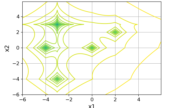
The graph of lines of equal levels of the above function will be as follows:


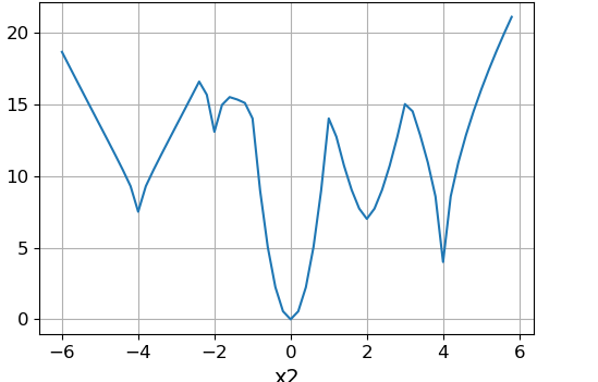
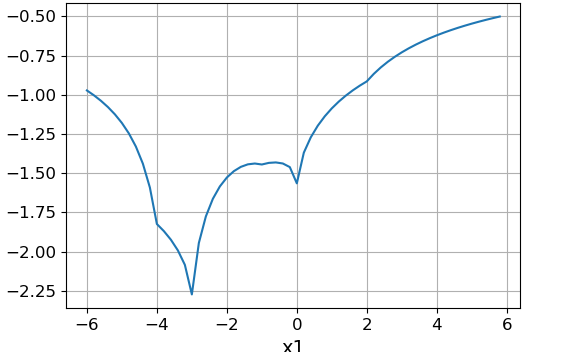
Slice function when$$ $ inline $ x_1 = x_2 $ inline $ :


Slice function when$$ $ inline $ x_2 = 4 $ inline $ :


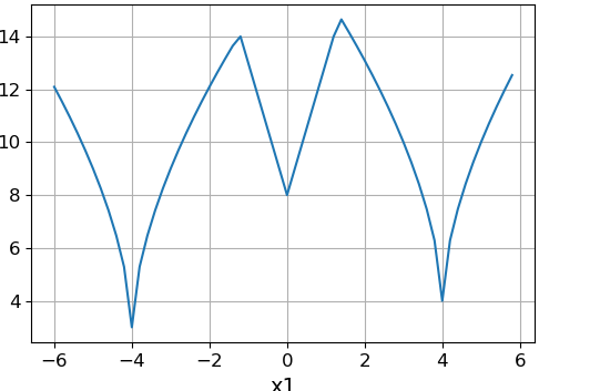
The above function has minima at the points: (0, 0), (-2, 0), (0, -2), (0, 4), (2, 2), (4, 0), (4, 4 ), (-4, 4), (-4, -4), (3, -5). The minimum is global at the point (0, 0).
Code to generate test functions:

def get_test_function_method_min(n: int, a: List[List[float]], c: List[List[float]], p: List[List[float]], b: List[float]): """ :param n:   :param a:    ,   ,    /      :param c:    :param p:       :param b:    :return:  ,       ,          """ def func(x): l = [] for i in range(n): res = 0 for j in range(len(x)): res = res + a[i][j] * np.abs(x[j] - c[i][j]) ** p[i][j] res = res + b[i] l.append(res) res = np.array(l) return np.min(res) return func 

Hyperbolic potential functions

The single-extremal function is:

$$$$ display $$ I_ {Y, i} (x-c_i) = - \ frac {1} {b_i * \ sum_ {j = 1} ^ m a_ {ij} | x_j-c {ij} | ^ {p_ {ij}} + d_i}, b_i> 0, d_i> 0 $$ display $$

This function also has a minimum at the point$$ $ inline $ c_i $ inline $ its depth is determined by$$ $ inline $ d_i $ inline $ . The degree of slope is given by the coefficient$$ $ inline $ b_i $ inline $ the bigger it is, the narrower the area of ​​the extremum and the steeper the function.

To obtain a multi-extremal function, it is necessary to apply the summation operator:

$$$$ display $$ I (x) = \ sum_ {i = 1} ^ N I_ {Y, i} (x-c_i) $$ display $$

Example:


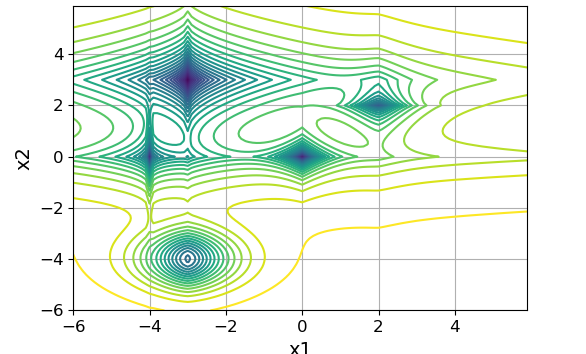
The graph of lines of equal levels of the above function will be as follows:


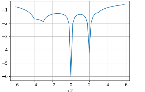
Slice function when$$ $ inline $ x_1 = x_2 $ inline $ :


Slice function when$$ $ inline $ x_2 = x_1 + 3 $ inline $ :


The above function has minimum points: (-4, 0), (0, 0), (-3, 3), (2, 2), (-3, -4). Global is the minimum at the point (-3, 3).

Under the spoiler is the code for generating a test function with additive modular functions in the denominator.

Exponential Potential Functions

The single-extremal function is:

$$$$ display $$ I_ {E, i} (x-c_i) = - d_i * exp \ {-b_i * sum_ {j = 1} ^ m a_ {ij} | x_j-c_ {ij} | ^ {p_ {ij}} \}, b_i> 0, d_i> 0 $$ display $$

Here all the letter designations carry the same meaning as in the previous method.
To obtain a multiextremal function, we also use the summation operator:

$$$$ display $$ I (x) = \ sum_ {i = 1} ^ N I_ {E, i} (x-c_i) $$ display $$

Example:


The graph of lines of equal levels is presented below:


Slice function when$$ $ inline $ x_1 = x_2 $ inline $ :


Slice function when$$ $ inline $ x_2 = -x_1 $ inline $ :


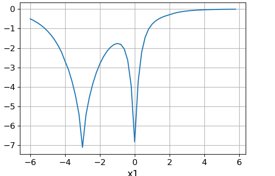
The above function has minimum points: (-4, 0), (0, 0), (-3, 3), (2, 2), (-3, -4). Global is the minimum at the point (-3, 3).


In addition to the above methods, harmonic functions can be used, however, their construction is a more complicated process. And the main disadvantage is the inability to control all local minima. You can also combine all of these methods to get even more complex functions.

Bibliography

Ruban A.I. Construction of multiextremal functions
Wikipedia. Test functions for optimization