Introduction

The ultimate goal of mathematical modeling in any field of knowledge is to obtain quantitative characteristics of the object under study. Some parameters of the gun, the shooting of which we modeled last time , were set in the problem statement: the initial velocity of the projectile, its caliber and the material from which it was made. The angle of inclination of the barrel can be attributed to varying parameters: any serious weapon allows for tip-over, including in the vertical plane.



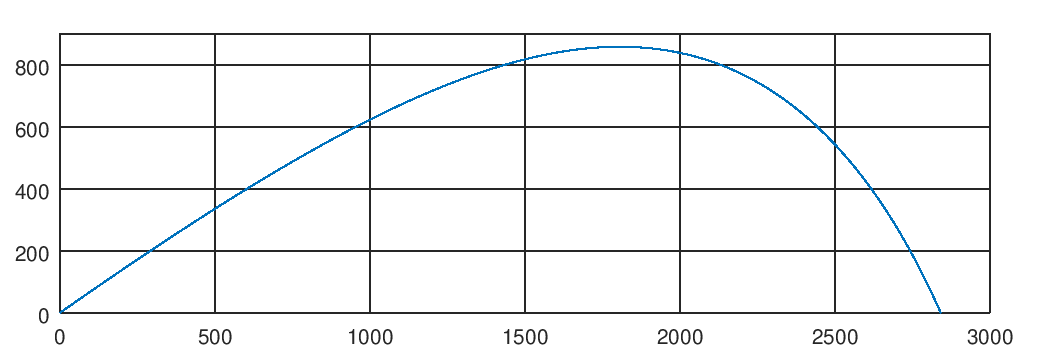
At the exit, we received the trajectory of the projectile, which gives us a rough idea of ​​the characteristics of the gun: with the given parameters, we got a firing range of just over 2.5 km and a height of projectile lifting just above 800 meters. More precisely, we can not say, or rather we can, if with a pencil on the grid we determine the coordinates of the necessary points on the graph. But this, as is known, is not our method. It would be nice to get this data with the accuracy provided by the tools we use and without manual labor. Here we will talk about it today.

1. Statement of the problem

So, the mathematical model constructed last time allows us, for any moment of time, to determine the coordinates and velocity of the projectile. In essence, we obtained functions that allow us to calculate the following trajectory parameters:
')

$$

$$\ begin {align} & x = x (t) \\ & y = y (t) \\ & v_x = v_x (t) \\ & v_y = v_y (t) \ end {align}$$

as a function of time. The height of the projectile is y (t). If we determine at which point in time the height becomes zero, then we solve the equation

$$

$$y (t) = 0$$

regarding time then we will find a moment in time $$$t ^ {*}$in which the projectile fell to the ground. Coordinate $$$x (t ^ {*})$and will be the range of the projectile.

How to find the maximum height of the projectile? From the trajectory plot, it is clear that as the projectile rises, its trajectory becomes more and more flat, while at the extreme point the speed momentarily becomes horizontal and the projectile moves further down.



In the language of mathematics, it is necessary to find the extremum point of the function $$$y = y (t)$. And what should be done for this? Equate its derivative to zero! In this case, the time derivative, that is, to solve the equation

$$

$$\ dot y (t) = 0$$

or

$$

$$v_y (t) = 0$$

for the derivative of the vertical coordinate with respect to time is the vertical projection of velocity. Root of this equation $$$t ^ {**}$there is a point in time when the projectile reaches its maximum height. Accordingly, we are interested in height

$$

$$h _ {\ max} = y (t ^ {**})$$

Simply? More than.

2. Equation, which is not

And here the kitten Gava is known to be in trouble. To begin with, even if the equation is given as a formula (analytically) it is not always possible to find its solution. For example

$$

$$x + 2 = e ^ {x}$$

How do you? Simple, but try to find the X, using all the things you were taught in school. That's the same ...


The solution of such an equation will have to be found numerically, especially since its graphical solution is obvious.


In the case of the gun model, everything is somewhat more cunning - our equation is not even defined by a formula. It is set, roughly speaking, by a table of phase coordinate values ​​obtained for quite specific parameters of the shot. We have no equation!

Well, no one bothers us, damn it, build this equation. But, before you start writing scripts, I want to apologize to the reader that I misled him. You can place several functions in one Octave script file, and the file name must necessarily match the function name. It is enough that the script does not begin with the definition of the function .

Create a new script in the same directory where the files ballistics.m, fm and f_air.m are located. Let's call it, for example cannon.m. To begin with, let's set the parameters of the projectile, the initial velocity and the direction of the shot.

%------------------------------------------------------------------------------- %   %------------------------------------------------------------------------------- %    global gamma = 7800; %    ( ) global c_f = 0.47; %  global d = 0.1; %------------------------------------------------------------------------------- %   %------------------------------------------------------------------------------- %   global v0 = 400; %     ( !) global alpha = 35; 

And now we will write a function that will calculate the phase coordinate values ​​for an arbitrary point in time.

 %------------------------------------------------------------------------------- %         %------------------------------------------------------------------------------- function Y = MotionOdeSolve(v0, alpha, t) %   x0 = 0; y0 = 0; vx0 = v0 * cos(deg2rad(alpha)); vy0 = v0 * sin(deg2rad(alpha)); Y0 = [x0; y0; vx0; vy0]; %    solv = lsode("f_air", Y0, [0; t]); %        t Y = [solv(2,1); solv(2,2); solv(2,3); solv(2,4)]; endfunction 

Please note that now we take only two values ​​as the moments of time passed to the function of solving the equation: the initial moment of time (t = 0) and the moment of time of interest to us. Accordingly, the solv variable will contain two phase coordinate vectors: the initial one and the one we need. We collect all the components of the end point of the phase trajectory into the vector Y and return its value from the function.

Now it costs us nothing to determine the dependence of the height of the projectile flight on time

 %------------------------------------------------------------------------------- %         %------------------------------------------------------------------------------- function h = height(t) global v0; global alpha; Y = MotionOdeSolve(v0, alpha, t); h = Y(2); endfunction 

Let's test the resulting function

 t1 = 10; t2 = 20; printf("h(%f) = %f, h(%f) = %f\n", t1, height(t1), t2, height(t2)); 

When you run the script for execution, we will see the following output in the command window

 >> cannon h(10.000000) = 855.013452, h(20.000000) = 500.106649 

Great, the function works! Similarly, we define the function of calculating the horizontal range

 %------------------------------------------------------------------------------- %         t %------------------------------------------------------------------------------- function d = dist(t) global v0; global alpha; Y = MotionOdeSolve(v0, alpha, t); d = Y(1); endfunction 

It can be seen that to calculate the height and range, we each time integrate the equations of motion, from the initial moment of time to the point of interest. In this way, we get a dependency that is not expressed by a specific formula. This is pretty cool.

3. Principles of numerical solution of nonlinear equations

Methods for the numerical solution of nonlinear and transcendental equations sharpened by solving equations of the form

$$

$$f (x) = 0$$

This form is easy to bring any equation. for example

$$

$$x + 2 = e ^ {x}$$

turns into

$$

$$x + 2 - e ^ {x} = 0$$

Where $$$f (x) = x + 2 - e ^ {x}$. The roots of this equivalent equation are equal to the roots of the original one. If we plot the function f (x), we will see such a picture.


the roots of the equation are the argument values ​​at those points where the graph intersects the x axis.

All methods for the numerical solution of such equations include two steps:

1. Search for the initial approximation of the root
2. Correction of the root with a given error

The initial approximation is understood to mean the value of the argument f (x), as close as possible to the root, or close enough to ensure the convergence of the method in a reasonable number of iterations.

The simplest method is the simple iteration method . To apply this method, the equation is converted to

$$

$$x = \ varphi (x)$$

and perform calculations on a recurrent formula

$$

$$x_ {i + 1} = \ varphi (x_i)$$

In our example

$$

$$x_ {i + 1} = e ^ {x_i} - 2$$

Let's look at the schedule. The equation has two roots. Find the leftmost root, choosing as the initial approximation $$$x_0 = -2$

$$

$$\ begin {align} & x_1 = e ^ {x_0} - 2 = e ^ {- 2} - 2 = -1.8647 \\ & x_2 = e ^ {x_1} - 2 = e ^ {- 1.8647} - 2 = -1.8451 \\ & x_3 = e ^ {x_2} - 2 = e ^ {- 1.8451} - 2 = -1.8412 \\ & x_4 = e ^ {x_3} - 2 = e ^ {- 1.8412} - 2 = -1.8415 \\ & x_5 = e ^ {x_4} - 2 = e ^ {- 1.8415} - 2 = -1.8414 \\ & x_6 = e ^ {x_5} - 2 = e ^ {- 1.8414} - 2 = -1.8414 \ end {align}$$

Aha, it is clear that starting with the sixth iteration, the fourth character of the resulting number remains unchanged. So we found the root of the equation with an error of less than 10 ^-4 in the sixth iteration.

Everything would be fine, but the method of simple iterations does not always converge. Try to find the second root of this equation, asking any, arbitrarily close initial approximation - you will not work: every new value will go farther and farther from the root. Convergence of the method can be achieved, there are ways, but in practice it makes life difficult for us. Therefore, to find the second root, apply another method. We expand the function under investigation into a Taylor series, in the vicinity of the initial approximation

$$

$$f (x) = f (x_0) + f '(x_0) \, (x - x_0) + \ frac {1} {2} \, f' '(x_0) \, (x - x_0) ^ 2 + ...$$

We confine ourselves to members of the first order of smallness, replacing the function f (x) itself with the tangent to its graph at the point x ₀

$$

$$f (x) \ approx f (x_0) + f '(x_0) \, (x - x_0)$$

and equating the resulting expression to zero, we solve it with respect to x

$$

$$x_1 = x_0 - \ frac {f (x_0)} {f '(x_0)}$$

We obtain an iterative formula

$$

$$x_ {i + 1} = x_i - \ frac {f (x_i)} {f '(x_i)}$$

In our example

$$

$$\ begin {align} & f (x) = x + 2 - e ^ {x} \\ & f '(x) = 1 - e ^ {x} \ end {align}$$

iterative formula

$$

$$x_ {i + 1} = x_ {i} - \ frac {x_i + 2 - e ^ {x_i}} {1 - e ^ {x_i}}$$

As an initial approximation, we take $$$x_0 = 1.0$and trying to iterate

$$

$$\ begin {align} & x_1 = x_0 - \ frac {x_0 + 2 - e ^ {x_0}} {1 - e ^ {x_0}} = 1 - \ frac {1 + 2 - e} {1 - e} = 1.1640 \\ & x_2 = x_1 - \ frac {x_1 + 2 - e ^ {x_1}} {1 - e ^ {x_1}} = 1.1640 - \ frac {1.1640 + 2 - e ^ {1.1640}} {1 - e ^ {1.1640}} = 1.1464 \\ & x_3 = x_2 - \ frac {x_2 + 2 - e ^ {x_2}} {1 - e ^ {x_2}} = 1.1464 - \ frac {1.1464 + 2 - e ^ {1.1464}} {1 - e ^ {1.1464}} = 1.1462 \\ & x_4 = x_3 - \ frac {x_3 + 2 - e ^ {x_3}} {1 - e ^ {x_3}} = 1.1462 - \ frac {1.1462 + 2 - e ^ {1.1462}} {1 - e ^ {1.1462}} = 1.1462 \ end {align}$$

As can be seen, this method has converged in four iterations with an accuracy of four characters. This method is called the Newton method . Its advantage is fast convergence. Among the shortcomings: high sensitivity to the accuracy of the initial approximation and the need to calculate the derivative of the left side of the equation. In the case when there is no analytical expression for the equation, one has to resort to the vile operation of numerical differentiation, which is not always convenient and possible.

I gave these examples in order to explain the general principle. In addition to these two methods, there are also a lot of methods, for example:

• Bisection method - it is characterized by guaranteed convergence, however, with a rather low speed
• Chord method - does not require calculation of the derivative of the function, has a good convergence rate

All the above methods require preliminary preparation, in the form of a search for the initial approximation or isolation interval of the root - the interval for changing the argument f (x), at the boundaries of which the function changes sign. In this case, it is safe to say (assuming the continuity of the function!) That there is at least one root inside the isolation interval.

4. Determine the parameters of the trajectory of the cannonball

So, we find the moment in time when the projectile will fall to the ground. First of all, we define the root isolation interval

 % %      .    % height(t) = 0 %  . % %     t0 = 0; deltaT = 1.0; t = t0; while (height(t) >= 0) t = t + deltaT; endwhile b = t; a = t - deltaT; %    t1 = t - deltaT / 2; 

We do this on the basis of the physical meaning of the task — after an immediately shot, the height of the projectile’s flight is non-negative. We iterate over all points in time, starting from zero, until the height becomes negative. We go over with a sufficiently large step (1 second) so that the procedure is not too long, because at each step we will re-integrate the differential equations of motion, which is very expensive in terms of computational costs. As soon as the height becomes negative, we end the search. The root of the equation h (t) = 0 is somewhere inside the interval [a, b]. The initial approximation is taken in the middle of this interval.

$$

$$t_1 = \ frac {a + b} {2} = t - \ frac {\ Delta t} {2}$$

Now we give the equation to eat the procedure for solving non-linear equations Octave

 %   t_end = fsolve("height", t1); 

The fsolve () function on input accepts a function describing the left side of the equation f (x) = 0 and the value of the initial approximation. Returns the root value calculated with a given accuracy. With what accuracy? Until we ask this question and use the default settings, at this stage they suit us.

Having obtained the value of the moment of time of the fall, we calculate the distance from the shooting position

 %    d_max = dist(t_end); %     printf("Shot distance: %f, m\n", d_max); 

Similarly, we find the time moment when the vertical projection of speed is zeroed and we calculate the height of the projectile at that moment

 %------------------------------------------------------------------------------- %      %------------------------------------------------------------------------------- function v = vy(t) global v0; global alpha; Y = MotionOdeSolve(v0, alpha, t); v = Y(4); endfunction % %       .   %  % % vy(t) = 0 % %     t = t0; while (vy(t) >= 0) t = t + deltaT; endwhile %    t1 = t - deltaT / 2; %   t_hmax = fsolve("vy", t1); %      h_max = height(t_hmax); printf("Maximal height: %f, m\n", h_max); 

In the command window you can see the results of the program.

 >> cannon h(10.000000) = 855.013452, h(20.000000) = 500.106649 Shot distance: 2840.991508, m Maximal height: 857.963929, m 

and also see how accurately the equations were solved

 >> height(t_end) ans = -1.2328e-06 >> vy(t_hmax) ans = 4.5117e-09 

For our educational purposes, accuracy is perfectly acceptable.

Conclusion

Today we have considered, in spite of the simplicity of the example, a rather wide layer of tasks. We now know that the absence of analytical dependencies describing a process is by no means an obstacle to the study of its characteristics. The unresolved was the task of determining the maximum firing range available for a given gun, but about this another time. Thanks for attention!