Introduction

I hope that you and I have gained enough experience to simulate something more serious than the flight of a stone. I propose such a task

A gun firing spherical cores tells them the initial speed of 400 m / s. Determine the trajectory of the projectile when shooting at an angle of 35 degrees to the horizon. The gravity field is considered to be uniform, neglecting the curvature of the Earth.

')


I must say, this is an example of an incorrectly assigned task. First, it does not say we consider, or do not take into account air resistance. And if we take into account, then the problem clearly lacks the parameters. Unfortunately, this kind of problem statement is a very common phenomenon. Therefore, we will solve the problem for both cases, and enter the necessary parameters into it ourselves. At the same time we will learn something new. Go!

1. Design scheme

Last time I deliberately did not draw any schemes to practice your imagination. It is easy to imagine a stone falling vertically down. Now the task is more difficult, and we cannot do without a drawing.



Such drawings are called a design diagram — a conditional graphical depiction of a process or object, made with regard to the assumptions entered into the task.

Please note that the diagram shows an arbitrary position of the projectile, into which it will fall after some time from the start of the movement. In problems of dynamics, it is more convenient to imagine the mutual arrangement of the force vectors and correctly decompose them into axial projections. The only thing we showed in the initial position is the initial velocity vector. This is useful when setting the initial conditions.

2. The formalization of the problem (without taking into account the resistance of the medium)

Everything is ready for a system of differential equations of motion.

$$

$$\ begin {align} & m \, \ ddot x = 0 \\ & m \, \ ddot y = -m \, g \ end {align}$$

We do not take into account air resistance, and we have only one force: it is projected on the x axis to zero, on the y axis - to the true value with a minus. After all, we have assumed that the field of gravity is uniform and the Earth is flat. So the force of gravity is always constant and directed vertically downwards. As you can see, nothing depends on the mass, the mass is reduced in both equations

$$

$$\ begin {align} & \ ddot x = 0 \\ & \ ddot y = -g \ end {align}$$

The result was a system of two second-order equations. We need to bring it to the form of Cauchy. Remember what it is? If you remember, try to do it yourself, without looking under the spoiler

3. Octave scripts, or how not to do the same work again

Last time, we entered commands directly into the Octave console. Well, the task we had was small. And if big? And if you want to change the parameters? And if you want to return to the postponed work? And if ... In short, it’s good to be able to save your programs on Octave. And yet there is nothing impossible.

At the bottom of the screen, under the command window there are tabs: Command Window, Editor and Documentation. Editor tab - what we need. This is an m-language script editor. Open this tab and enter such text into it.

%------------------------------------------------------------------------------- % %       %    % %------------------------------------------------------------------------------- function dYdt = f(Y, t) g = 9.81; %    dYdt(1) = Y(3); % dx/dt = vx dYdt(2) = Y(4); % dy/dt = vy dYdt(3) = 0; % dvx/dt = 0 dYdt(4) = -g; % dvy/dt = -g endfunction 

This is nothing but the right side of the system of differential equations of projectile motion, in our problem, designed as a function in the m-language. The meaning is the same as last time. Only now we have four equations. Well, the acceleration of free fall is taken as a normal, adult value. Save this file on disk as fm

Attention! Each function in the m-language requires saving to its own file, the name of which coincides with the name of the function. In our case, the function has the name f, which means the file has the name f.



What are the lines starting with "%"? And this, apache brothers, comments! The text preceded by this character in Octave is ignored by the interpreter. Comments are not only possible, but you need to supply your programs in order to at least navigate in them yourself, not to mention other people who want to use your program.

So, we set the octave system of equations. Create a new file, name it, for example, ballistics.m and save it in the same place where you saved the previous file. Let's start to solve the problem!

 %------------------------------------------------------------------------------- %   %------------------------------------------------------------------------------- %    v0 = 400; %       alpha = 35 * pi / 180; %------------------------------------------------------------------------------- %   %------------------------------------------------------------------------------- x0 = 0; y0 = 0; vx0 = v0 * cos(alpha); vy0 = v0 * sin(alpha); Y0 = [x0; y0; vx0; vy0]; %------------------------------------------------------------------------------- %    %------------------------------------------------------------------------------- %    t0 = 0; %    tend = 10.0; %    deltaT = 0.1; %      t = [t0:deltaT:tend]; %     Y = lsode("f", Y0, t); %     plot(Y(:,1), Y(:,2)); 

The meaning of most operations is clear from the comments. Separately, I will explain the initial conditions. We have four phase coordinates: two Cartesian coordinates of the projectile, two projections of its velocity on the coordinate axes

$$

$$\ begin {align} & Y (1) \ to x (t) \\ & Y (2) \ to y (t) \\ & Y (3) \ to v_x (t) \\ & Y (4) \ to v_y ( t) \ end {align}$$

For each of the phase coordinates, you must specify their initial value. It is logical to set the initial position at the origin. As for the other two variables, this is the attention, the initial values ​​of the projections of the velocity vector on the x and y axes . Then I drew the initial velocity vector so that it was easy to find its projections on the axes

$$

$$\ begin {align} & v_x = v_0 \, \ cos \ alpha \\ & v_y = v_0 \, \ sin \ alpha \\ \ end {align}$$

Now everything is ready. Click on the button with the gear and the yellow triangle to run the script. In response, the system will give a window



ask us to add the path that the script lies in the script search path. This must be done once after loading the script into the editor or creating a new script. Click the button "Add ..." and get the result



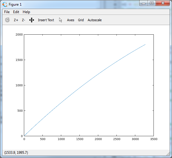
Looks promising. Time 10 seconds is not enough for the outfit to land. Change the value of tend and run the script again until we get a similar picture.



corresponding tend = 47 seconds. The simulation is over, the projectile has flown below the x-axis, but this is normal, because we do not simulate its meeting with the surface.

4. The formalization of the problem (taking into account the resistance of the medium)

The ball as a form of projectile, we chose not by chance. As it does not turn, it has the same section from all sides - a circle (by the way, the same reason the Vostok spacecraft had a spherical shape of the descent vehicle). So, no matter how direct the air flow, when flowing around the force of resistance to movement will be the same and equal to

$$

$$R = c_f \, S \, \ frac {\ rho \, v ^ 2} {2}$$

where c _f = 0.47 is the form drag coefficient; S is the cross-sectional area; $$$\ rho$= 1.29 kg / m ³ - air density; v is the flow velocity, in our case, the velocity of the projectile.

The force vector of resistance will always be directed against the velocity vector. Therefore, we will redraw the design scheme



How to take into account the fact that for any moment of time the vector $$$\ vec R$directed against speed? Very simple. We know that the velocity vector is tangential to the trajectory. We introduce a vector $$$\ vec \ tau$with a length of 1 and directed to the same direction as the speed. Then vector $$$\ vec R$can be expressed through vector $$$\ vec \ tau$and modulus of resistance

$$

$$\ vec R = - R \, \ vec \ tau$$

How to find a vector $$$\ vec \ tau$? Very simply, its projections on the coordinate axes will be equal.

$$

$$\ begin {align} \ tau_x = \ frac {v_x} {v} \\ \ tau_y = \ frac {v_y} {v} \ end {align}$$

The velocity vector module is easily expressed through its projection.

$$

$$v = \ sqrt {v_x ^ 2 + v_y ^ 2}$$

Then the projections of the vector of the air resistance force on the coordinate axes are easy to calculate

$$

$$\ begin {align} & R_x = - R \, \ tau_x = -R \, \ frac {v_x} {v} = - \ frac {1} {2} \, c_f \, S \, \ rho \, v \, v_x \\ & R_y = - R \, \ tau_y = -R \, \ frac {v_y} {v} = - \ frac {1} {2} \, c_f \, S \, \ rho \, v \ , v_y \\ \ end {align}$$

And it changes the equations of motion.

$$

$$\ begin {align} & m \, \ ddot x = - \ frac {1} {2} \, c_f \, S \, \ rho \, v \, v_x \\ & m \, \ ddot y = - \ frac {1} {2} \, c_f \, S \, \ rho \, v \, v_y - m \, g \ end {align}$$

This is what comes out, the mass is no longer reduced? Yes, now the dynamics of the flight of the projectile will depend on the mass. But nobody forbids dividing the mass; we divide both equations into it

$$

$$\ begin {align} & \ ddot x = - k \, v \, v_x \\ & \ ddot y = - k \, v \, v_y - g \ end {align}$$

Where

$$

$$k = \ frac {c_f \, S \, \ rho} {2 \, m}$$

coefficient determining the contribution of the resistance force to the acceleration of the projectile. It can be greatly simplified if we recall that the shell is a ball

$$

$$m = \ gamma \, V = \ gamma \, \ frac {4} {3} \, \ pi \, r ^ 3, \ quad S = \ pi \, r ^ 2$$

The first formula is the mass of the ball, and here $$$\ gamma$Is the density of the material from which the core is made, and r is the radius of the core. The second formula is the cross-sectional area of ​​the ball. Substitute these formulas into the expression for the coefficient and simplify

$$

$$k = c_f \, \ rho \ frac {\ pi \, r ^ 2} {\ frac {8} {3} \, \ gamma \, \ pi \, r ^ 3} = \ frac {3} {8 } \, \ frac {c_f \, \ rho} {r \, \ gamma} = \ frac {3} {4} \, \ frac {c_f \, \ rho} {d \, \ gamma}$$

where d is the diameter of the core, the caliber of our gun. From this formula it is already clear that the larger the caliber and the denser the material of the projectile, the less the influence of the air resistance will be.

Let us set the parameters of the projectile. Add the following lines to the end of the file ballistics.m

 %------------------------------------------------------------------------------- %   %------------------------------------------------------------------------------- %    global gamma = 7800; %    ( ) global c_f = 0.47; %  global d = 0.1; 

Let the core be cast iron caliber 100 mm. What a word is global in front of each variable. Thus, we say to the system that the variables created will be accessible to all scripts and the functions defined in them, that is, they will be global.

It remains to write for Octave the model we have constructed as a function, let it be the f_air function. Naturally, for it you need to create a separate file f_air.m. Try it yourself. I will give a hint: the beginning of the body of this function should be determined once again by our global parameters of the projectile, but without values. This is necessary for the function to see global variables.

 global c_f; global gamma; global d; 

If it is very difficult, look under the spoiler.



Now we solve the system of equations of motion, in the file ballistics.m we give the commands

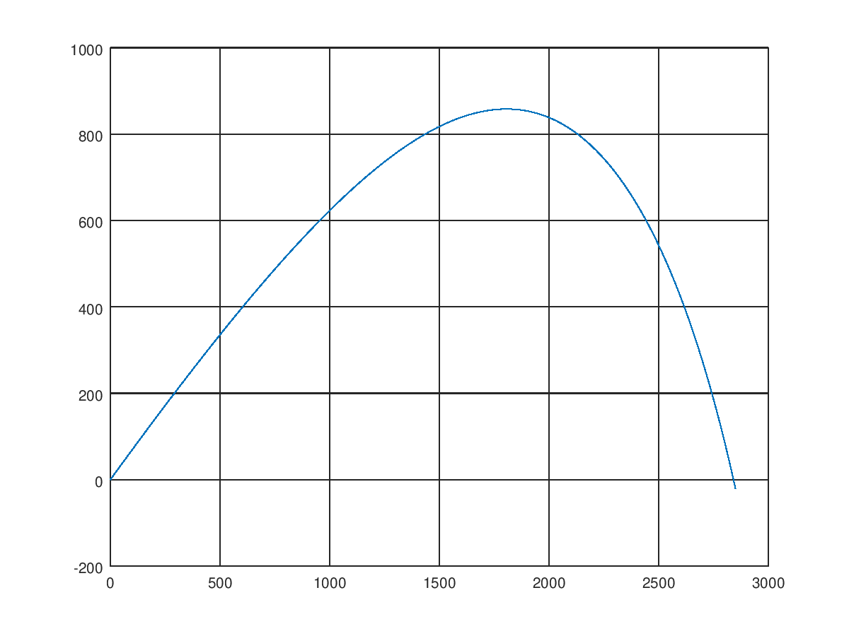
 Y_air = lsode("f_air", Y0, t); plot(Y_air(:,1), Y_air(:,2)); 

that is, we integrate new equations of motion with the same initial conditions and on the same time interval as for the problem without taking air resistance into account, as well as draw a trajectory graph



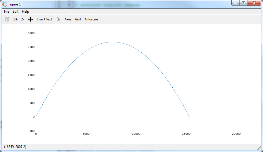
Wow, the maximum flight altitude has decreased quite significantly. And 47 seconds is now too much range, the projectile falls to the ground much earlier. Play with time



With tend = 26 seconds we see that the range is quite significant. It can be seen that the aerodynamic drag has a very significant effect on the characteristics of our gun and, in reality, it cannot be neglected. The shape of the trajectory also changes: it is more shelter on the ascending part, and it goes steeply down on the descending one, a little resembling an ideal parabola.

5. Comparison of the trajectories of the projectile

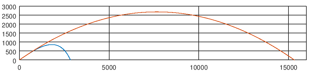
We already see that the results of the simulation of the flight of the nucleus differ from each other. But everything is known in visual comparison. We construct two trajectories simultaneously. Can? Yes, simple

 %    plot(Y_air(:,1), Y_air(:,2), Y(:,1), Y(:,2)); 

First, we specified the abscissa and the ordinate for one trajectory, then for the other. What happened?



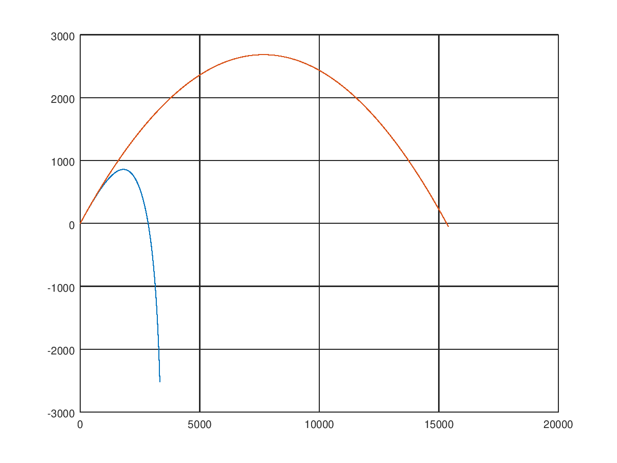
Um, this is some kind of nonsense. That's right, the time of flight of the projectile in different solutions is different. We do not model collision of a nucleus with a surface. You can get out of this situation by setting the limits of coordinate changes along the axes of the command axis (), like this

 %        xmin = 0; xmax = 16000; ymin = 0; ymax = 3000; axis([xmin xmax ymin ymax], "manual"); 

Now the graphics will look like this.



Already better. At least the trajectories can be compared with each other. And if we want the same scale on all axes? Googling gave such a command

 set(gca,'dataaspectratio',[1 1 1]); 

defining the same scale of the axes of the graph along all axes



Under the spoiler, the full text of the file ballistics.m

Conclusion

In the example we have considered, we are faced with the fundamental property of the laws of nature - they are non-linear. If air resistance is taken into account, then the phase coordinates right in the part of differential equations enter nonlinearly. There is no analytical solution, that is, a problem expressed in elementary functions. The presence of an analytical solution for real-life engineering problems is more likely an exception. And without modeling in their decision can not do.

But by itself, solving equations of motion in practice makes little sense. What did this decision give us? Yes, we saw the influence of the air resistance force on the flight of a cannonball. But we, for example, did not answer many questions, for example, what is the exact firing range of our gun? What is the maximum height of the projectile? At what angle should you shoot in order to reach the maximum range?

Mathematical models are created in order to solve practical problems of technology with the help of them. This is what we'll talk about next time.

PS: Sample projects will now be available on Github