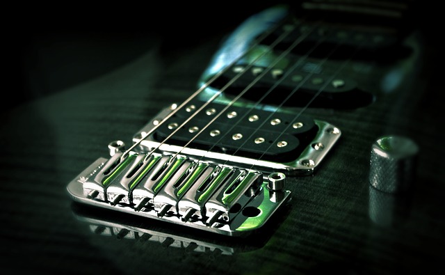
Measuring and shaping the frequency characteristics of electric guitars
Let's talk about art. For example, about music. For example, about guitars.
Creating electric guitars is a fairly conservative thing. Despite the tremendous advances in signal processing , which allow you to get any sounds in real time from the guitars ( JTV89 ), the very “warm and tube” sound that the guitar should have by itself is still quite appreciated. On the other hand, with all of this, the sound of the guitar should have exactly the characteristics that the customer wants, who suddenly wanted to have some kind of specific sound from their guitar.
The sound of a guitar is shaped by the following things:
')
For those strings that will be used by the person, the creator of the guitar, of course, is not responsible. The effect of body parts on the sound for electric (non-acoustic) pieces is quite religious. The influence of this, on the one hand, is not denied, but on the other hand, no one really knows how to take this into account (and even if he says he knows, most likely he will not be able to explain anything properly).
Pickups remain. Their position and signal transmission characteristics. This we can measure, compare and take into account. On these issues there is a fairly developed and simple theoretical base.
The theoretical basis for assessing the influence of the position of the sensor can be found here . A simple theoretical description of the transfer characteristics of the sensor here . For my part, I will try to retell it all as short as possible so that you do not read English.
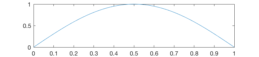
Guitar string is a string that is tied at two ends. When we jerk her, she starts to vibrate, because she is tied and she can not escape anywhere. But there are important aspects of how this happens. The string vibrates with different periods. Periods of a multiple of the length of the string: 1, ½, ¼,…, ... This can be represented with the following picture:
You can conduct an experiment with the guitar yourself by carefully looking at the picture. Pull the string, and then gently touch with your finger in the middle of the string. As can be understood from the picture, such a movement will drown out all the odd harmonics in which there is not a minimum in this place, and the sound will not disappear, but will change somewhat. This technique is called natural flageolet , if you pull the string by already holding your finger in the middle and tapping the flageolet , if you pull the string, and then touch your finger. But this is the lyrics. It is important to us that there are many frequencies and, in fact, everything is not limited to periods that are multiples of the string length.
And here we need to remember that the pickup creates a magnetic field in the vicinity of the string. The metal string oscillates in this field directly above the sensor and perturbs it somehow. Due to this, a current is generated in the sensor circuit in accordance with the Faraday law. And all the speeds of the string directly above the sensor are interesting to us.
Physicists have found that the relative (normalized) speed of movement of a string over some place of a string is described by the following formula:
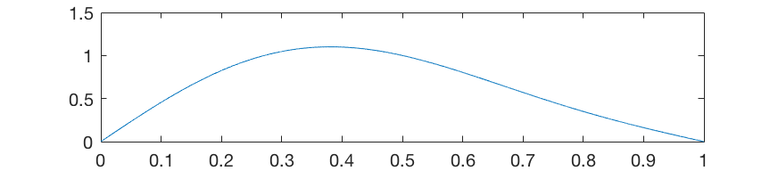
Note on distance x . If the string oscillated with only one main harmonic, the maximum of this magnitude would be exactly at the center of the string (sine pi is equal to 1 in half)
However, the string has the rest of the harmonics, and the intensity of the harmonics falls in proportion to the square of their number, the second is four times weaker, the third at nine, and so on. Even adding a second harmonic will change the speed of the string and make its distribution asymmetric:
And if you add up “all” harmonics, the maximum will shift to a position exactly ⅓ from the nut.
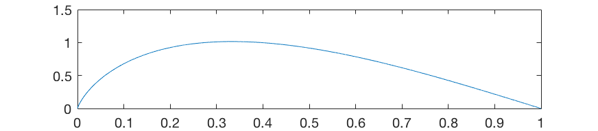
This fact determines the position of the sensors and the resonator hole on the body of the guitar.
And back to the topic. Each string has its main frequency F 0 , and the main length of the string is L 0 . It is obvious that changes in frequency with a change in the sounding “length” will be inversely proportional to the fundamental frequencies (the longer, the lower the frequency):
You can take this and substitute in equation 1.
The theoretical response of the "perception" of the string sensor with zero width. Picture from here
On the logarithmic scale of frequencies, the sine amplitude graph looks pretty mysterious and unusual ... But then from formula (2) it is obvious that when X is changed, this whole picture will shift to the right / left relative to the frequency axis. This, in fact, forms the characteristic sounds of the bridge and neck sensors (there is a picture, as it is located) . For the bridge, the first peak leaves to the right, for the neck to the left. For bridge, X is very small, so F must be much larger to reach the first peak. Thus, the bridge is characterized by a less bass sound and more midrange.
This could be stopped with the position of the sensor, but that's not all.
The sensor is not the point above the guitar from which the sound is taken. The sensor has a width. Those. The sensor “collects” and adds the sound above the “set” of points above itself, for each of which the frequency response is slightly shifted. Or with clever words - the integral is taken along the entire length of the intersection of the sensor and the string ( here those who are not afraid of integrals ). And from this integral we get that we have not one sine, but two. Both depend on the frequency and one depends on X, and the other on the width of the sensor W.
Theoretical phase of the "perception" of the string sensor with a finite width. Picture from http://www.till.com/articles/PickupResponse/
It looks like this mathematically:
where, k is a string-dependent constant. It is clear that W (sometimes much) is less than X, even taking into account division by 2, so the graph has another peak, which shifts strongly to high frequencies.
And here we have some bad holes in the frequency response (CH) in the most unpleasant places. If we expand W, on the one hand, holes in the black-hole will disappear, but the signal amplitude will decrease, because in the formula (3) the denominator is W. In general, there is some problem that, oddly enough, is solved automatically.
We talked a lot about where the sensor stands. But very little about how he conducts the signal. The sensor is a second-order RLC-circuit with a resonance and its black-tone looks like this:
ChH of a typical sensor as a second-order resonant circuit. Picture from www.muzique.com/lab/pickups.htm
The resonant peak quite gracefully covers some of the holes formed by the fact that the sensor is wide. And the whole art of creating a guitar is that no notes especially do not have dips in loudness, and there are peaks in the right places. In this article, however, we will not say anything special about it. This can be measured, for example, as follows .
And now, when you roughly understand what is happening, in fact, we will tell what we measured and what we received.
We were interested to know, and how the sound coming out of the guitar is different from the one that sounds when you pull the string.
To determine this, we took the microphone Shure M58. Due to its popularity, its approximate frequency response is everywhere. Thus, we could measure the “real sound” (which is determined by the string and the body). Then they put the microphone in front of the sensor (at the optimum distance for recording). Pull the string. The microphone recorded what is determined by points (3.4) from the first part, and to the sensor by all four. Then it remains only to somehow "subtract" the sound recorded from the microphone from the sound recorded from the sensor and see what the sensor actually does with the sound, apart from what the sound is, what the guitar is made of, and what strings are on it. We wrote a program that can do all this and build all sorts of graphics.
In fact, everything is not so simple, but about it at the end.
A little walk through some parts of the process.
The selection takes place on an extremely simple principle: Where we have a signal on average more than a certain limit value over a sufficiently large amount of time, then we also have a note.
For this we:
All notes are recorded with different volume and volume from the microphone and from the sensor differ. Therefore, now it is necessary to align all this in order to be able to compare. For this we:
After each of the trimming is normalized, a Fourier is taken from it and its spectrum is calculated. In the spectrum a lot of superfluous, from which we must get rid of. For example, actually, the played note, which has large, but highly variable, amplitudes. To do this, we first find all these peaks. How?
The spectrum of the MI notes of the first octave and how it is smoothed
Further, with respect to each peak, we replace ± M points of the original series with points of the smoothed and shifted series. In principle, it was possible to immediately take the smoothed, but you never know something important can be missed.
Thus, we get the series "without peaks" for both the microphone and the sensor.
Subtracting each other the resulting sensor and microphone rows and then averaging them, we get something like this:
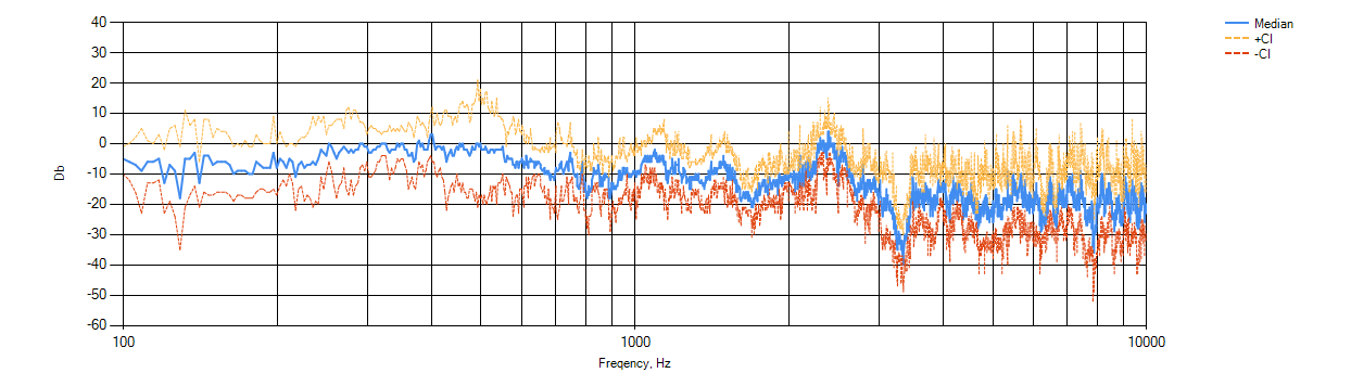
ChX Neck sensor copy JP7 (in a sense, the transfer function of the sensor).
CI +, CI- is a plus / minute confidence interval for the average series. It is important here to understand that the specific values of decibels are not as important as the relative location. We do not know what “really” was the volume of the string. The microphone could stand on, could closer. The normalization of loudness made the volume integrally similar, but we do not know if they really were. Therefore, the signature of the Y axis is largely because it is ugly not to sign the axis. The y axis does not carry any sacramental meaning. However, it is sometimes interesting to see how the signal of the microphone and the sensor correlate when they are drawn separately:
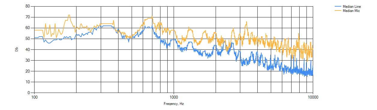
Smoothed spectra for the JP7 Neck copy sensor. Spectra are drawn averaged and smoothed.
But again, we must remember that these graphs can be safely moved relative to each other up and down.
And why did you really need this whole theory before the graphs? How are these things related? This is where the most interesting lies.
Let's consider the PM for JP7 and the same theoretical, calculated for the neck length of 650 mm, the distance of the sensor from the lower nut is 130 mm (neck), the sensor width is 2 inches (51 mm), and for Mi of the first octave 328 Hz:
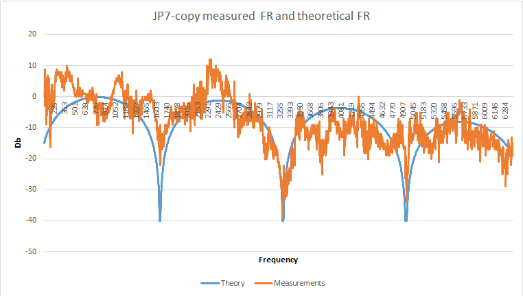
We clearly see how the theoretical failures associated with the location of the sensor coincide. sin (pi * 129.5 * 1620 / (640 * 328)) is approximately equal to 0 and this is half the period, exactly as in the graph. In the region of 4800 Hz, the failure is less, because it is there that is (most likely) the resonance of the transfer function of the electrical part of the sensor.
It is not always so obvious.
Take another guitar. Fender Stratocaster Ritchie Blackmore Edition. A rather characteristic guitar with specific properties and sensors with the complex name Seymour Duncan Quarter Pound Flat SSL-4 single-coil Strat pickup. Consider its received frequency response. The length of the neck is 655 mm, the distance of the sensor from the lower nut is 150 mm (neck), the width of the sensor is 2 inches (50 mm) (in fact, there is a very, very powerful single , and the parameters of the humbucker are better suited for it), and for Mi first 328 Hz octaves:
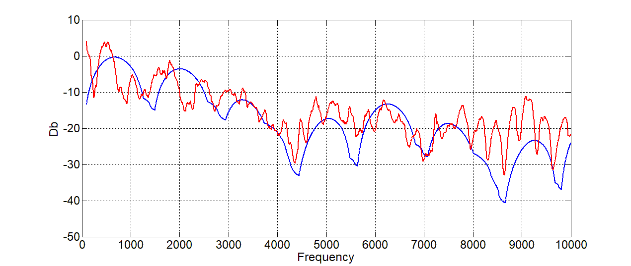
I must say that this did not happen immediately, but when applying a low-pass filter to the theory. And in general, the effect of some other strange things is visible.
Look at the same fender. You can also compare, for example, neck (150 mm) sensor c bridge (50 mm) sensor. We measure the characteristic of the first, the characteristic of the second, then we look at a separate graph (after a little filtering).
Green on the chart - bridge, orange - neck. From the graph you can see exactly that, and so everything seems to know how. Neck pulls out very low frequencies, Bridge medium-high. The questions here, as usual, arise in details that are of interest only to great lovers of music and all that. For example, in the neck peaks around 9000 Hz.
Now, about why "in fact everything is not so simple . "
The microphone, especially the directional one, also removes only a part of the string, like the sensor, respectively, has a similar FM, depending on the position of the microphone and the “width” of the sound capture. However, it is obvious that at the microphone the “width” of the sensor is much larger, respectively, all the sine frequencies are much larger and the microphone's frequency response is largely expressed in the form of high-frequency oscillations “noise” in the spectrum.
Take, for example, the frequency response of the Fender Stratocaster Ritchie Blackmore Edition, measured for the neck position of the sensor. Since the ChH is described by a sine (as we know it from theory), we can once again take the transform from the Fourier spectrum to estimate the frequencies that are allocated (taking the Fourier from the spectrum is a very dubious entertainment, by the way). The result is shown in the picture.
Fourier spectrum transform Fender Stratocaster Ritchie Blackmore Edition (neck)
The peaks are clearly defined, defined by the properties of the “sensor position”, “sensor width” and “microphone width”. Most likely there is no strongly marked peak “microphone position”, because the microphone was right in front of the sensor ...
For the single, it does not affect exactly the way. For the humbucker, everything is done in such a way that around 9000 there is a failure. And this also forms the corporate “not bright” sound of such a pickup. Although, of course, this is not the only thing that influences the sound of such a sensor;
Coauthor: A.A. Gorodetsky, Imperial College London.
PS We publish our articles on several runet sites. Subscribe to our pages on the VK , FB or Telegram channel to learn about all our publications and other news from Maxilect.
Creating electric guitars is a fairly conservative thing. Despite the tremendous advances in signal processing , which allow you to get any sounds in real time from the guitars ( JTV89 ), the very “warm and tube” sound that the guitar should have by itself is still quite appreciated. On the other hand, with all of this, the sound of the guitar should have exactly the characteristics that the customer wants, who suddenly wanted to have some kind of specific sound from their guitar.
The sound of a guitar is shaped by the following things:
')
- Pickup position
- Pickup characteristics
- Type of strings
- Resonant properties of the hull and materials
For those strings that will be used by the person, the creator of the guitar, of course, is not responsible. The effect of body parts on the sound for electric (non-acoustic) pieces is quite religious. The influence of this, on the one hand, is not denied, but on the other hand, no one really knows how to take this into account (and even if he says he knows, most likely he will not be able to explain anything properly).
Pickups remain. Their position and signal transmission characteristics. This we can measure, compare and take into account. On these issues there is a fairly developed and simple theoretical base.
Theoretical part
The theoretical basis for assessing the influence of the position of the sensor can be found here . A simple theoretical description of the transfer characteristics of the sensor here . For my part, I will try to retell it all as short as possible so that you do not read English.
Guitar string is a string that is tied at two ends. When we jerk her, she starts to vibrate, because she is tied and she can not escape anywhere. But there are important aspects of how this happens. The string vibrates with different periods. Periods of a multiple of the length of the string: 1, ½, ¼,…, ... This can be represented with the following picture:
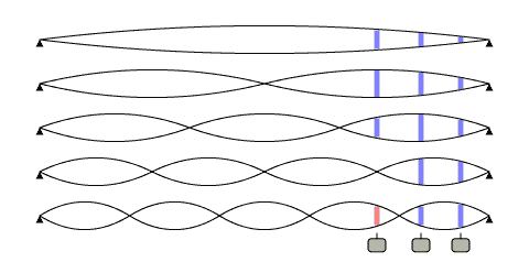 Harmonics strings. Picture from www.till.com/articles/PickupResponse |  |
You can conduct an experiment with the guitar yourself by carefully looking at the picture. Pull the string, and then gently touch with your finger in the middle of the string. As can be understood from the picture, such a movement will drown out all the odd harmonics in which there is not a minimum in this place, and the sound will not disappear, but will change somewhat. This technique is called natural flageolet , if you pull the string by already holding your finger in the middle and tapping the flageolet , if you pull the string, and then touch your finger. But this is the lyrics. It is important to us that there are many frequencies and, in fact, everything is not limited to periods that are multiples of the string length.
And here we need to remember that the pickup creates a magnetic field in the vicinity of the string. The metal string oscillates in this field directly above the sensor and perturbs it somehow. Due to this, a current is generated in the sensor circuit in accordance with the Faraday law. And all the speeds of the string directly above the sensor are interesting to us.
Physicists have found that the relative (normalized) speed of movement of a string over some place of a string is described by the following formula:
X is the distance from the nut (lower) to the pickup, L is the length of the vibrating part of the string (there are some reservations, but we omit them).
Note on distance x . If the string oscillated with only one main harmonic, the maximum of this magnitude would be exactly at the center of the string (sine pi is equal to 1 in half)
However, the string has the rest of the harmonics, and the intensity of the harmonics falls in proportion to the square of their number, the second is four times weaker, the third at nine, and so on. Even adding a second harmonic will change the speed of the string and make its distribution asymmetric:
And if you add up “all” harmonics, the maximum will shift to a position exactly ⅓ from the nut.
This fact determines the position of the sensors and the resonator hole on the body of the guitar.
And back to the topic. Each string has its main frequency F 0 , and the main length of the string is L 0 . It is obvious that changes in frequency with a change in the sounding “length” will be inversely proportional to the fundamental frequencies (the longer, the lower the frequency):
You can take this and substitute in equation 1.
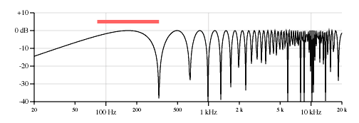
Here - constant, provided that the sensor is above one place of the string, and it turns out that the speed is sinusoidally frequency dependent. Naturally, the speed sign does not interest us, so you can draw this dependence in decibels, as in the above article:
The theoretical response of the "perception" of the string sensor with zero width. Picture from here
On the logarithmic scale of frequencies, the sine amplitude graph looks pretty mysterious and unusual ... But then from formula (2) it is obvious that when X is changed, this whole picture will shift to the right / left relative to the frequency axis. This, in fact, forms the characteristic sounds of the bridge and neck sensors (there is a picture, as it is located) . For the bridge, the first peak leaves to the right, for the neck to the left. For bridge, X is very small, so F must be much larger to reach the first peak. Thus, the bridge is characterized by a less bass sound and more midrange.
This could be stopped with the position of the sensor, but that's not all.
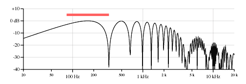
The sensor is not the point above the guitar from which the sound is taken. The sensor has a width. Those. The sensor “collects” and adds the sound above the “set” of points above itself, for each of which the frequency response is slightly shifted. Or with clever words - the integral is taken along the entire length of the intersection of the sensor and the string ( here those who are not afraid of integrals ). And from this integral we get that we have not one sine, but two. Both depend on the frequency and one depends on X, and the other on the width of the sensor W.
Theoretical phase of the "perception" of the string sensor with a finite width. Picture from http://www.till.com/articles/PickupResponse/
It looks like this mathematically:
where, k is a string-dependent constant. It is clear that W (sometimes much) is less than X, even taking into account division by 2, so the graph has another peak, which shifts strongly to high frequencies.
And here we have some bad holes in the frequency response (CH) in the most unpleasant places. If we expand W, on the one hand, holes in the black-hole will disappear, but the signal amplitude will decrease, because in the formula (3) the denominator is W. In general, there is some problem that, oddly enough, is solved automatically.
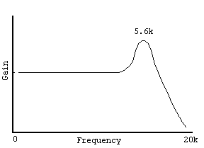
We talked a lot about where the sensor stands. But very little about how he conducts the signal. The sensor is a second-order RLC-circuit with a resonance and its black-tone looks like this:
ChH of a typical sensor as a second-order resonant circuit. Picture from www.muzique.com/lab/pickups.htm
The resonant peak quite gracefully covers some of the holes formed by the fact that the sensor is wide. And the whole art of creating a guitar is that no notes especially do not have dips in loudness, and there are peaks in the right places. In this article, however, we will not say anything special about it. This can be measured, for example, as follows .
And now, when you roughly understand what is happening, in fact, we will tell what we measured and what we received.
Installation and processing algorithm
We were interested to know, and how the sound coming out of the guitar is different from the one that sounds when you pull the string.
Two words about installation and measurement
To determine this, we took the microphone Shure M58. Due to its popularity, its approximate frequency response is everywhere. Thus, we could measure the “real sound” (which is determined by the string and the body). Then they put the microphone in front of the sensor (at the optimum distance for recording). Pull the string. The microphone recorded what is determined by points (3.4) from the first part, and to the sensor by all four. Then it remains only to somehow "subtract" the sound recorded from the microphone from the sound recorded from the sensor and see what the sensor actually does with the sound, apart from what the sound is, what the guitar is made of, and what strings are on it. We wrote a program that can do all this and build all sorts of graphics.
In fact, everything is not so simple, but about it at the end.
What devices and software, we repeat again?
- Sound card EMU 0204
- Shure M58 Microphone
- Fender Stratocaster Ritchie Blackmore Edition
- master copy of Music Man JP7
- Program for automatic signal processing in C # (NAudio, MathNet)
- Additional analysis: Excel, Matlab
Algorithm
- We record the microphone in the left channel, turn on the guitar in the right line (EMU allows it).
- We pull for one string N times, so that “identical” signals are recorded in the sensor and microphone and there is something to average. We make sure that there are gaps of silence between the notes.
- We remove the noise and slightly align the signals to the eye (but this is not necessary)
- We select from record each individual recorded note in two arrays: a note from a microphone, a note from a sensor.
- We normalize all arrays with records so that notes have the same “power per unit time”
- For each array, we do the Fourier transform N = 32768 (but 16384 can be different, nothing too)
- Select the peaks in the spectra of the arrays, which correspond to the sound of the note itself and smooth it (Oddly enough, it is the note itself that doesn’t help us much in the evaluations)
- Deduct each spectrum of a microphone from each spectrum (taking into account the microphone's own frequency response).
- We average the results for all frequencies, obtaining a spectrum that characterizes the difference between the sound from the sensor and the sound recorded on the microphone.
A little walk through some parts of the process.
Selection of significant parts of the record
The selection takes place on an extremely simple principle: Where we have a signal on average more than a certain limit value over a sufficiently large amount of time, then we also have a note.
For this we:
- We take the absolute values of the sensor signal;
- We add the constant C (so that there is no zero, because then it is necessary to logarithm);
- We translate into decibels;
- Smooth by moving average ;
- We pass through the entire array, selecting pieces, where the signal is greater than some constant Lim;
- Fold back too short pieces;
- We believe that the signal from the sensor is in the same place as the microphone, so the microphone signal is cut off along the same boundaries.
- We return two arrays containing “sliced” notes.
Normalization
All notes are recorded with different volume and volume from the microphone and from the sensor differ. Therefore, now it is necessary to align all this in order to be able to compare. For this we:
- We take the reference "scrap" and for it we consider the "power per unit time":
Where, N - the size of the i -th array, r - values from the i -th array.
- Then for each i-th "trim" recalculate the values of the array:
Harmonics
After each of the trimming is normalized, a Fourier is taken from it and its spectrum is calculated. In the spectrum a lot of superfluous, from which we must get rid of. For example, actually, the played note, which has large, but highly variable, amplitudes. To do this, we first find all these peaks. How?
- For the whole spectrum, we make double smoothing with a moving average with a coefficient of 0.05.
- Smoothing makes the series lagging behind the original, because in the moving average, the “prehistory” of any point begins to matter. To avoid this, the offset is found by checking the correlation of the original series and the smoothed one. Such an offset is chosen that makes this correlation maximum.
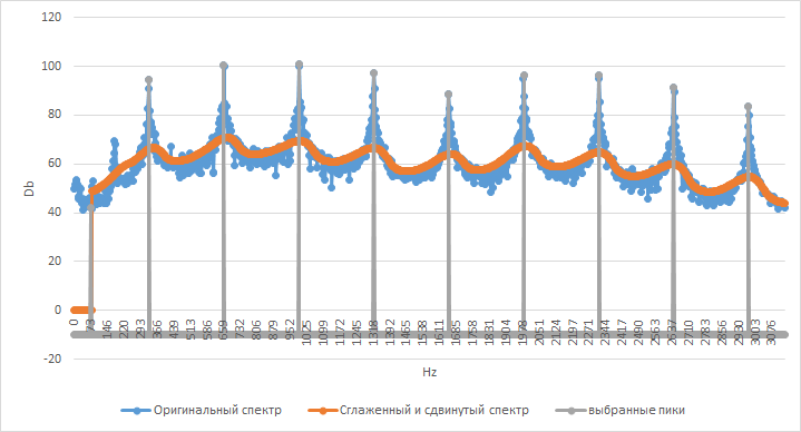
- After that, there are continuous arrays of points that exceed the smoothed and shifted schedule by 1.5 standard deviations of the original series and the maximum is taken from them. It looks like this:
The spectrum of the MI notes of the first octave and how it is smoothed
Further, with respect to each peak, we replace ± M points of the original series with points of the smoothed and shifted series. In principle, it was possible to immediately take the smoothed, but you never know something important can be missed.
Thus, we get the series "without peaks" for both the microphone and the sensor.
Receive frequency response
Subtracting each other the resulting sensor and microphone rows and then averaging them, we get something like this:
ChX Neck sensor copy JP7 (in a sense, the transfer function of the sensor).
CI +, CI- is a plus / minute confidence interval for the average series. It is important here to understand that the specific values of decibels are not as important as the relative location. We do not know what “really” was the volume of the string. The microphone could stand on, could closer. The normalization of loudness made the volume integrally similar, but we do not know if they really were. Therefore, the signature of the Y axis is largely because it is ugly not to sign the axis. The y axis does not carry any sacramental meaning. However, it is sometimes interesting to see how the signal of the microphone and the sensor correlate when they are drawn separately:
Smoothed spectra for the JP7 Neck copy sensor. Spectra are drawn averaged and smoothed.
But again, we must remember that these graphs can be safely moved relative to each other up and down.
Back to theory
And why did you really need this whole theory before the graphs? How are these things related? This is where the most interesting lies.
Let's consider the PM for JP7 and the same theoretical, calculated for the neck length of 650 mm, the distance of the sensor from the lower nut is 130 mm (neck), the sensor width is 2 inches (51 mm), and for Mi of the first octave 328 Hz:
We clearly see how the theoretical failures associated with the location of the sensor coincide. sin (pi * 129.5 * 1620 / (640 * 328)) is approximately equal to 0 and this is half the period, exactly as in the graph. In the region of 4800 Hz, the failure is less, because it is there that is (most likely) the resonance of the transfer function of the electrical part of the sensor.
It is not always so obvious.
Take another guitar. Fender Stratocaster Ritchie Blackmore Edition. A rather characteristic guitar with specific properties and sensors with the complex name Seymour Duncan Quarter Pound Flat SSL-4 single-coil Strat pickup. Consider its received frequency response. The length of the neck is 655 mm, the distance of the sensor from the lower nut is 150 mm (neck), the width of the sensor is 2 inches (50 mm) (in fact, there is a very, very powerful single , and the parameters of the humbucker are better suited for it), and for Mi first 328 Hz octaves:
I must say that this did not happen immediately, but when applying a low-pass filter to the theory. And in general, the effect of some other strange things is visible.
And what else can you compare?
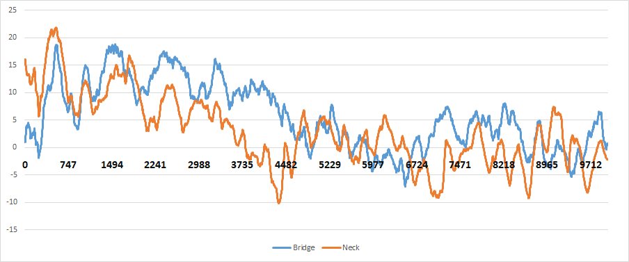
Look at the same fender. You can also compare, for example, neck (150 mm) sensor c bridge (50 mm) sensor. We measure the characteristic of the first, the characteristic of the second, then we look at a separate graph (after a little filtering).
Green on the chart - bridge, orange - neck. From the graph you can see exactly that, and so everything seems to know how. Neck pulls out very low frequencies, Bridge medium-high. The questions here, as usual, arise in details that are of interest only to great lovers of music and all that. For example, in the neck peaks around 9000 Hz.
Reservations
Now, about why "in fact everything is not so simple . "
The microphone, especially the directional one, also removes only a part of the string, like the sensor, respectively, has a similar FM, depending on the position of the microphone and the “width” of the sound capture. However, it is obvious that at the microphone the “width” of the sensor is much larger, respectively, all the sine frequencies are much larger and the microphone's frequency response is largely expressed in the form of high-frequency oscillations “noise” in the spectrum.
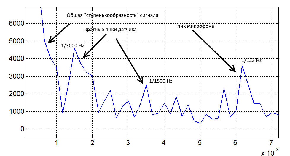
Take, for example, the frequency response of the Fender Stratocaster Ritchie Blackmore Edition, measured for the neck position of the sensor. Since the ChH is described by a sine (as we know it from theory), we can once again take the transform from the Fourier spectrum to estimate the frequencies that are allocated (taking the Fourier from the spectrum is a very dubious entertainment, by the way). The result is shown in the picture.
Fourier spectrum transform Fender Stratocaster Ritchie Blackmore Edition (neck)
The peaks are clearly defined, defined by the properties of the “sensor position”, “sensor width” and “microphone width”. Most likely there is no strongly marked peak “microphone position”, because the microphone was right in front of the sensor ...
Conclusions for those who like conclusions
- The position of the sensor affects no less than its own frequency response. And maybe even more;
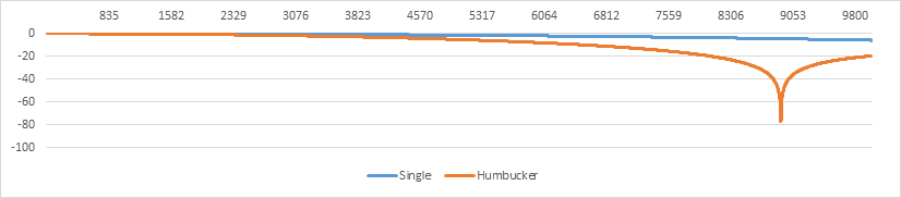
- The width of the sensor, based on the formula (3), affects exactly as shown in the picture.
For the single, it does not affect exactly the way. For the humbucker, everything is done in such a way that around 9000 there is a failure. And this also forms the corporate “not bright” sound of such a pickup. Although, of course, this is not the only thing that influences the sound of such a sensor;
- It is impossible to put the sensor in such a way (or make it so wide) that it does not kill any frequencies. Actually, these dead frequencies set the characteristic sound of the guitar;
- If you want some specific sound from the ordered guitar, it is important to find out who you heard this sound from, then it will be easier to focus on the position of the sensors on that instrument.
- In principle, one can easily dare and theoretically build some of his own filters from combinations of positions, widths and electrical circuits of sensors. Apply these filters to a sound recorded on a microphone and watch - do you like it? Do you want the guitar to sound that way? Are you ready to look for the perfect sound?
Coauthor: A.A. Gorodetsky, Imperial College London.
PS We publish our articles on several runet sites. Subscribe to our pages on the VK , FB or Telegram channel to learn about all our publications and other news from Maxilect.
Source: https://habr.com/ru/post/349236/
All Articles