How to make your code 80 times faster
All beaver!
We are starting the third set for the Python Developer course, which means that there is an open lesson in front of us, which partially replace the old-format open door days and where you can get acquainted with interesting material from our teachers, and that we found another interesting material . This time to speed up the "snake" code.
Go.
')
PyPy is able to speed up the code by 2 times, which pleases very many people. I want to share a short, personal story, proving that PyPy is capable of more.
DISCLAIMER: This is not a miracle cure for all occasions, yes, it worked specifically in this case, but it may not be as effective in many others. However, the method is still interesting. Moreover, the steps described here, I applied during development in the same manner, which makes the article a vital example of optimizing PyPy.
I experimented with evolutionary algorithms a few months ago: the plan was ambitious - to automatically develop logic capable of controlling (simulated) quadcopter, that is, the PID controller ( spoiler : does not fly).

The idea is that in the presence of a population of random creatures, in each generation the fittest survive and reproduce with small, random changes.
However, within the framework of this post, the initial task is not so important, so we move directly to the code. To control the quadcopter, the creature uses the
At first I tried to run the code on CPython; and here is the result:
That is ~ 6.15 seconds / generation, except for the first.
Then, I tried PyPy 5.9:
Oh! It turned out ~ 5.5 times slower than with CPython. In part, this was expected: nympy is based on cpyext, known for its slowness. (Actually, we are working on this - on the
Let's try to avoid cpyext. The first obvious step is to use numpypy instead of numpy (here’s a hack that allows you to use only part of the micronumpy). Check if the speed has improved:
On average, ~ 2.7 seconds: 12 times faster than PyPy + numpy and more than 2 times faster than the original CPython. Already, many would run to tell how good PyPy is.
But let's try to improve the result. As usual, let's analyze what it takes the most time. Here is the link to the vmprof profile . We spend a lot of time inside numpypy and allocate tons of temporary arrays to store the results of various operations.
In addition, we will look at the jit trace and find the run function: this is the loop in which we spend most of the time, it consists of 1796 operations. The operations for the line
An interesting implementation of the part
All this is not very optimal: in our case, it is known that the size of
The well-known compiler optimization - reversal of the loop will probably help to solve this problem. From the point of view of the compiler, a loop reversal is always accompanied by a risk - if the matrix is too large, you will end up with a large, shapeless mass of code that will be useless if the size of the array is constantly changing. This is one of the main reasons why PyPy JIT in this case is not even trying to do that.
However, we know that the matrix is small and always the same size. Therefore, we deploy the cycle manually:
The code additionally has a health check to make sure that the value is equal to that provided via
Let's check how it works. First with CPython:
It looks good - 60% faster than the original implementation of CPython + numpy. Check PyPy:
Yes, this is not a mistake. After a couple of generations, time stabilizes in the region of ~ 0.07-0.08 seconds per generation. Which is about 80 (eighty) times faster than the implementation of CPython + numpy, and 35-40 times faster than the naive PyPy + numpy.
Let's look at the trace again: there are no more expensive calls and no temporary malloc () 's. The root of the logic is in lines 386-416, where we see the execution of fast C-level multiplications and additions: float_mul and float_add are translated directly to the mulsd and addsd86 commands.
As I said, this is a very specific example, and this method is not universal: unfortunately, you should not wait for 80-fold acceleration of an arbitrary code. However, this clearly shows the potential of PyPy in high-speed computations. And most importantly, this is not a trial benchmark, designed specifically for good performance. PyPy is a small but realistic example.
How to reproduce the result
THE END
If anything, then we are waiting for questions here or at an open lesson .
We are starting the third set for the Python Developer course, which means that there is an open lesson in front of us, which partially replace the old-format open door days and where you can get acquainted with interesting material from our teachers, and that we found another interesting material . This time to speed up the "snake" code.
Go.
')
PyPy is able to speed up the code by 2 times, which pleases very many people. I want to share a short, personal story, proving that PyPy is capable of more.
DISCLAIMER: This is not a miracle cure for all occasions, yes, it worked specifically in this case, but it may not be as effective in many others. However, the method is still interesting. Moreover, the steps described here, I applied during development in the same manner, which makes the article a vital example of optimizing PyPy.
I experimented with evolutionary algorithms a few months ago: the plan was ambitious - to automatically develop logic capable of controlling (simulated) quadcopter, that is, the PID controller ( spoiler : does not fly).
The idea is that in the presence of a population of random creatures, in each generation the fittest survive and reproduce with small, random changes.
However, within the framework of this post, the initial task is not so important, so we move directly to the code. To control the quadcopter, the creature uses the
run_step method, which is run in each delta_t (full code): class Creature(object): INPUTS = 2 # z_setpoint, current z position OUTPUTS = 1 # PWM for all 4 motors STATE_VARS = 1 ... def run_step(self, inputs): # state: [state_vars ... inputs] # out_values: [state_vars, ... outputs] self.state[self.STATE_VARS:] = inputs out_values = np.dot(self.matrix, self.state) + self.constant self.state[:self.STATE_VARS] = out_values[:self.STATE_VARS] outputs = out_values[self.STATE_VARS:] return outputs - inputs - numpy array in which the final point and the current position along the Z axis are located;
- outputs - the numpy array in which the thrust is transmitted to the motors. For a start, all 4 motors are limited to the same pitch, so the quadrocopter moves up and down along the Z axis;
self.statecontains arbitrary values of unknown size that are passed from one step to another;self.matrixandself.constantcontain the logic itself. By transferring the “correct” values to them, theoretically, we could get a perfectly tuned PID controller. They randomly mutate between generations.
run_step is called at 100 Hz (in the virtual simulation time interval). The generation consists of 500 creatures, each of which we test for 12 virtual seconds. Thus, each generation contains 600,000 run_step executions.At first I tried to run the code on CPython; and here is the result:
$ python -m ev.main Generation 1: ... [population = 500] [12.06 secs] Generation 2: ... [population = 500] [6.13 secs] Generation 3: ... [population = 500] [6.11 secs] Generation 4: ... [population = 500] [6.09 secs] Generation 5: ... [population = 500] [6.18 secs] Generation 6: ... [population = 500] [6.26 secs] That is ~ 6.15 seconds / generation, except for the first.
Then, I tried PyPy 5.9:
$ pypy -m ev.main Generation 1: ... [population = 500] [63.90 secs] Generation 2: ... [population = 500] [33.92 secs] Generation 3: ... [population = 500] [34.21 secs] Generation 4: ... [population = 500] [33.75 secs] Oh! It turned out ~ 5.5 times slower than with CPython. In part, this was expected: nympy is based on cpyext, known for its slowness. (Actually, we are working on this - on the
cpyext-avoid-roundtrip brunch, the result is better than with CPython, but we'll talk about this in another post).Let's try to avoid cpyext. The first obvious step is to use numpypy instead of numpy (here’s a hack that allows you to use only part of the micronumpy). Check if the speed has improved:
$ pypy -m ev.main # using numpypy Generation 1: ... [population = 500] [5.60 secs] Generation 2: ... [population = 500] [2.90 secs] Generation 3: ... [population = 500] [2.78 secs] Generation 4: ... [population = 500] [2.69 secs] Generation 5: ... [population = 500] [2.72 secs] Generation 6: ... [population = 500] [2.73 secs] On average, ~ 2.7 seconds: 12 times faster than PyPy + numpy and more than 2 times faster than the original CPython. Already, many would run to tell how good PyPy is.
But let's try to improve the result. As usual, let's analyze what it takes the most time. Here is the link to the vmprof profile . We spend a lot of time inside numpypy and allocate tons of temporary arrays to store the results of various operations.
In addition, we will look at the jit trace and find the run function: this is the loop in which we spend most of the time, it consists of 1796 operations. The operations for the line
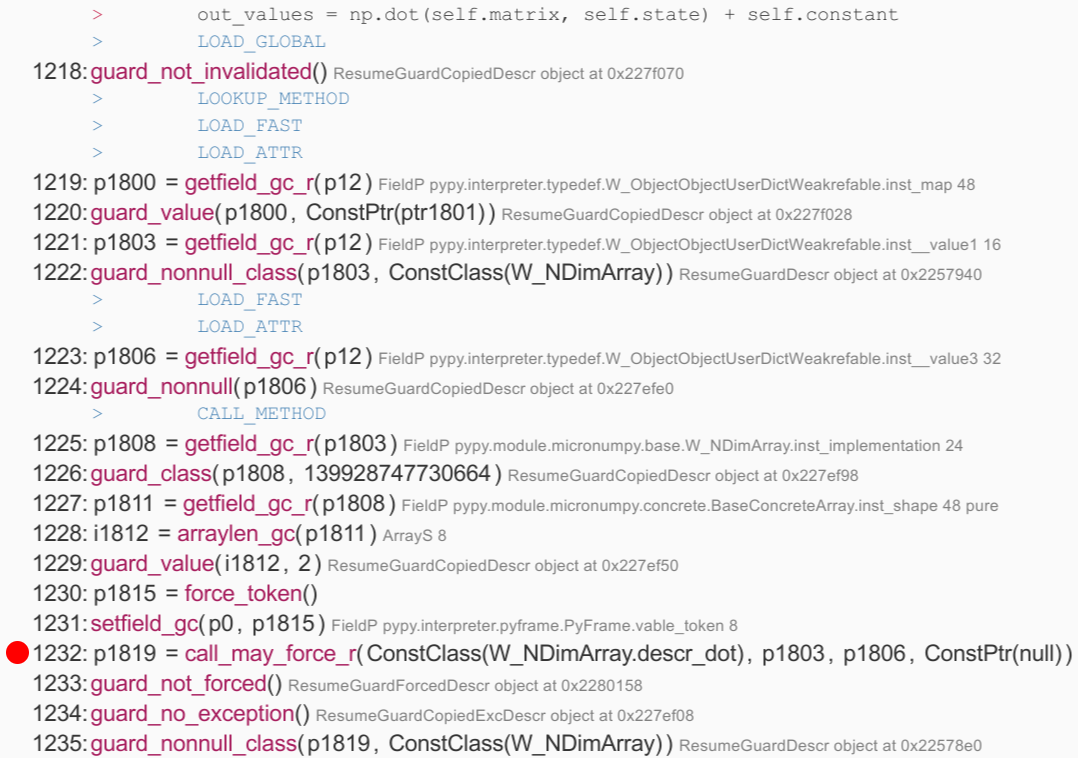
np.dot(...) + self.constant are between lines 1217 and 1456. Below is an excerpt calling np.dot(...) . Most of the operators cost nothing, but in line 1232 we see the RPython function call descr_dot ; on implementation, we see that it creates a new W_NDimArray to store the result, which means it will have to do malloc() :An interesting implementation of the part
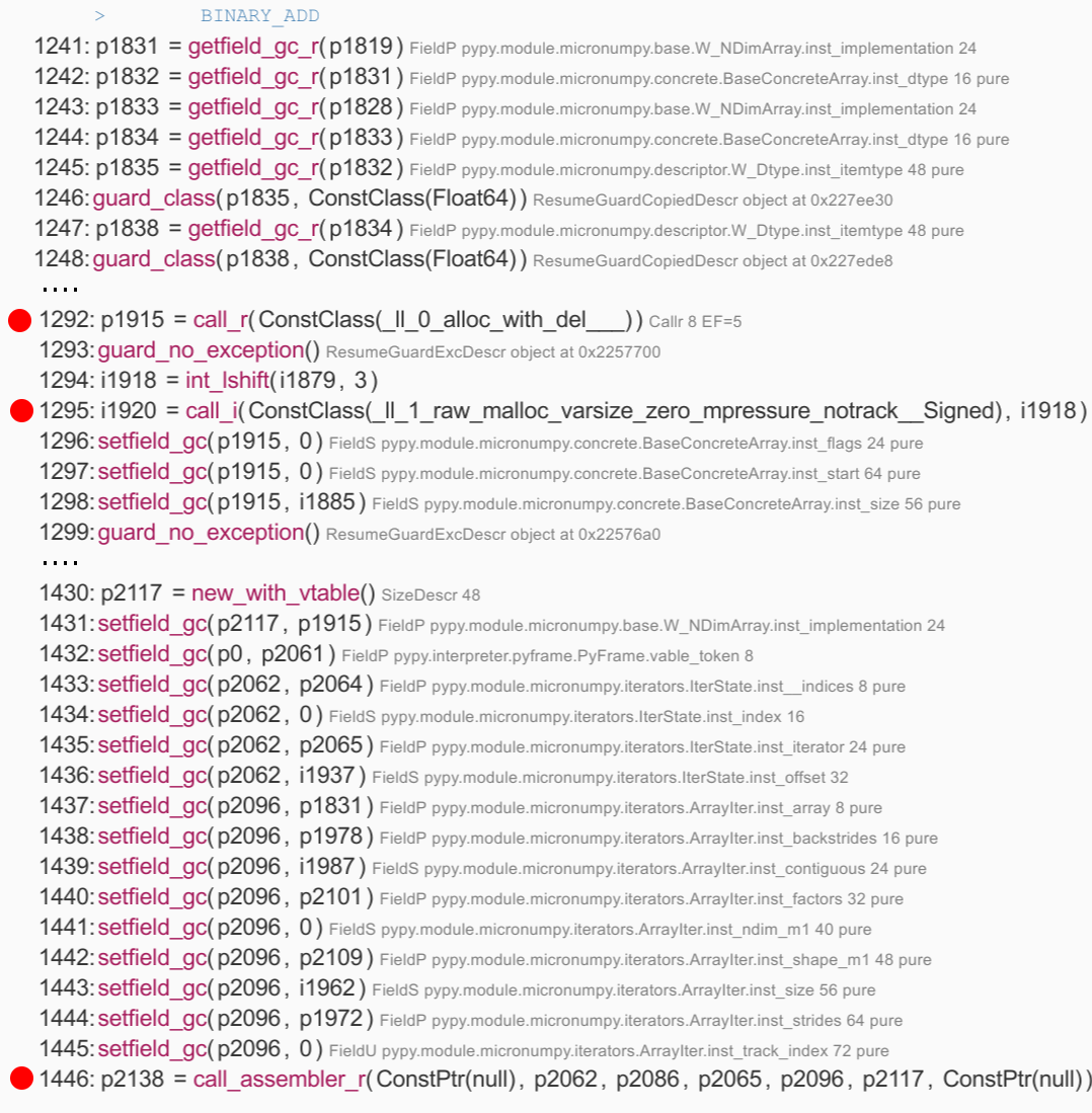
+ self.constant - the call to W_NDimArray.descr_add was embedded in JIT, so it is easier for us to understand what is happening. In particular, we see a call to __0_alloc_with_del____ , allocating W_NDimArray for the result, and aw_malloc, allocating the array itself. Then there is a long list of 149 simple operations that define the fields of the final array, create an iterator, and finally call acall_assembler — this is the actual logic to perform the addition, which JIT 'or separately. call_assembler one of the operations for making JIT-to-JIT calls:All this is not very optimal: in our case, it is known that the size of
self.matrix always (3, 2) - which means we do a lot of work, including 2 malloc() calls for temporary arrays, just to call two functions that the total amount is 6 multiplications and 6 additions. Note that this is not the fault of JIT: CPython + numpy having to do the same, but in hidden calls C.The well-known compiler optimization - reversal of the loop will probably help to solve this problem. From the point of view of the compiler, a loop reversal is always accompanied by a risk - if the matrix is too large, you will end up with a large, shapeless mass of code that will be useless if the size of the array is constantly changing. This is one of the main reasons why PyPy JIT in this case is not even trying to do that.
However, we know that the matrix is small and always the same size. Therefore, we deploy the cycle manually:
class SpecializedCreature(Creature): def __init__(self, *args, **kwargs): Creature.__init__(self, *args, **kwargs) # store the data in a plain Python list self.data = list(self.matrix.ravel()) + list(self.constant) self.data_state = [0.0] assert self.matrix.shape == (2, 3) assert len(self.data) == 8 def run_step(self, inputs): # state: [state_vars ... inputs] # out_values: [state_vars, ... outputs] k0, k1, k2, q0, q1, q2, c0, c1 = self.data s0 = self.data_state[0] z_sp, z = inputs # # compute the output out0 = s0*k0 + z_sp*k1 + z*k2 + c0 out1 = s0*q0 + z_sp*q1 + z*q2 + c1 # self.data_state[0] = out0 outputs = [out1] return outputs The code additionally has a health check to make sure that the value is equal to that provided via
Creature.run_step .Let's check how it works. First with CPython:
$ python -m ev.main Generation 1: ... [population = 500] [7.61 secs] Generation 2: ... [population = 500] [3.96 secs] Generation 3: ... [population = 500] [3.79 secs] Generation 4: ... [population = 500] [3.74 secs] Generation 5: ... [population = 500] [3.84 secs] Generation 6: ... [population = 500] [3.69 secs] It looks good - 60% faster than the original implementation of CPython + numpy. Check PyPy:
Generation 1: ... [population = 500] [0.39 secs] Generation 2: ... [population = 500] [0.10 secs] Generation 3: ... [population = 500] [0.11 secs] Generation 4: ... [population = 500] [0.09 secs] Generation 5: ... [population = 500] [0.08 secs] Generation 6: ... [population = 500] [0.12 secs] Generation 7: ... [population = 500] [0.09 secs] Generation 8: ... [population = 500] [0.08 secs] Generation 9: ... [population = 500] [0.08 secs] Generation 10: ... [population = 500] [0.08 secs] Generation 11: ... [population = 500] [0.08 secs] Generation 12: ... [population = 500] [0.07 secs] Generation 13: ... [population = 500] [0.07 secs] Generation 14: ... [population = 500] [0.08 secs] Generation 15: ... [population = 500] [0.07 secs] Yes, this is not a mistake. After a couple of generations, time stabilizes in the region of ~ 0.07-0.08 seconds per generation. Which is about 80 (eighty) times faster than the implementation of CPython + numpy, and 35-40 times faster than the naive PyPy + numpy.
Let's look at the trace again: there are no more expensive calls and no temporary malloc () 's. The root of the logic is in lines 386-416, where we see the execution of fast C-level multiplications and additions: float_mul and float_add are translated directly to the mulsd and addsd86 commands.
As I said, this is a very specific example, and this method is not universal: unfortunately, you should not wait for 80-fold acceleration of an arbitrary code. However, this clearly shows the potential of PyPy in high-speed computations. And most importantly, this is not a trial benchmark, designed specifically for good performance. PyPy is a small but realistic example.
How to reproduce the result
$ git clone https://github.com/antocuni/evolvingcopter $ cd evolvingcopter $ {python,pypy} -m ev.main --no-specialized --no-numpypy $ {python,pypy} -m ev.main --no-specialized $ {python,pypy} -m ev.main THE END
If anything, then we are waiting for questions here or at an open lesson .
Source: https://habr.com/ru/post/349230/
All Articles