Foreword

It is difficult to overestimate the importance of computer modeling in the modern world. Long ago, the times when the trajectories of launching satellites into near-earth orbit were calculated by a crowd of calculating girls with Felix at the ready (there was such a computer ). Today, a modest-sized box near your desktop solves all possible and unimaginable tasks. But there is one "but."



The state of engineering education, I don’t know how it is in the capitals, but here, on the periphery, it looks depressing in the context of this issue. The blame here is an approach to teaching in universities such disciplines as "Numerical methods for solving engineering problems on a computer", "Mathematical modeling in% you need to write% yourself" and others. This problem of engineering education arises from the fact that in courses similar to those listed, interdisciplinary communication is sometimes completely cut off. A trainee does not have a chain in his head: a fundamental theory -> practical application -> a tool for solving a problem.
')
I have long thought to write a cycle in which everything that we call modern mathematical modeling will be disassembled. But to do this is simple and affordable for those who are just beginning to learn this vast discipline of modern science. It is not known what will come of this, but I’m inviting those who find it interesting under cat.

1. Mathematical principles of natural philosophy

Yes, we start with the mechanics. The science of the pre-Newtonian era, in the modern sense, was incomplete. It lacked a clear, universal method of scientific research. But this does not mean that science did not exist. A huge reservoir of experimental data from different spheres of human activity was accumulated. Scientists solved complex problems, often using methods whose genius is still striking. But the brilliant discoveries were sporadic. Until a man appeared, he wrote a work that gave scientists a clear mathematical apparatus that became the main tool of scientific knowledge for centuries to come.

It was Newton's " Beginnings ... ", which laid the foundations of differential calculus with a practical approach in the direction of mechanics and made the latter the first in the history of this scientific theory. The laws of mechanics, somewhere successfully, somewhere not very, began to try to explain all the phenomena occurring in nature, from optics to electricity, from thermodynamics to the structure of matter. Time has dotted the "i", other theories have come to replace the mechanistic principles, and the mechanics themselves have evolved considerably. But at the same time, mechanics, like no other discipline, clearly and in detail illustrates all that we will discuss below. Most of the examples of this cycle will be somehow connected with the modeling of mechanical systems, at least in his first articles.

Before we begin, I have to give a few explanatory notes:

1. The reader should be familiar with the main content of the course of mathematics, to understand what vector values ​​are. Without this, no way. I will try to provide text links for detailed study of bottlenecks, but I will not go into details
   
2. As a tool for performing numerical calculations, we will rely on the GNU Octave package. Why - two reasons. It is free, is analogous to Matlab and contains everything you need for our purposes. The second reason - I want to get to know him, so let it be my whim)
   
3. The author is waiting for comments on the material presented in any form, whether it be comments, letters, etc. This will help make the material better.
   

2. Quantitative parameters describing the movement

Mechanics is a science that studies the movement of material bodies. Under the mechanical movement understand the movement of the body in space over time. This definition should lead you to the following questions:

1. What is meant by the body?
2. How to determine its position in space?

Under the body, in the scientific and philosophical sense, it is customary to understand any material object, but this vague definition is clearly not enough. Therefore, mechanics operate on the following abstract concepts:

1. Material point (or just "point")
2. Absolutely solid body (or simply “solid body”)

Under the point is commonly understood body, the size of which is neglected in specific conditions of motion. To make it clear, from the perspective of this definition, we will look at our planet moving around the Sun.



Earth has a diameter of about 13,000 kilometers. The sun - almost half a million kilometers. Wow point! But here the distance between them is 150 million kilometers, and the path traveled by the Earth in a year in orbit is about a billion kilometers. As we see, on such a scale of space, the Earth and the Sun can really be considered points.

And if we want to study the rotation of the Earth around its axis?



Then each point of the Earth moves along its own trajectory relative to the axis of rotation and cannot be neglected by its dimensions! Here, the Earth should be considered as a set of connected points or a solid body.

Thus, mechanics places at our disposal not the body itself, but its two simple models, using which most practical problems can be solved with the degree of accuracy required in practice.

It makes no sense to talk about a solid body without understanding how the point motion is described. Obviously, in order to determine the position of a point in space, it is necessary to choose a origin, for example, another point. Having determined the beginning of the reference, it is necessary to choose those parameters, the quantitative value of which will make it possible to estimate the position in space of the moving point of interest. Depending on which parameters are selected, I distinguish three ways of defining the movement of a point.

2.1. Vector way to set motion

It's very simple - from the origin O to point M they draw a vector. The length and direction of this vector allows us to judge where the point is located.



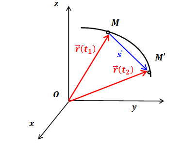
The point will move in space, the vector will change its length and direction, and its end will draw in space an imaginary curve, which is called the trajectory of the point. The vector itself is called the radius vector of the point. If we know the mathematical law, the formula by which we can calculate this vector for any moment of time, then we know the law of motion of a point

$$

$$\ vec r = \ vec r (t)$$

This entry tells us that the radius vector is a function of time.

2.2. Coordinate way of specifying the motion of a point

From the origin we can draw three mutually perpendicular axes x, y, and z. Then the position of the point will be determined by a triple of numbers - coordinates in the Cartesian system.



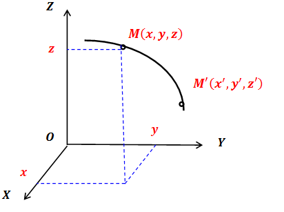
In this case, the law of motion of a point is three functions of time.

$$

$$\ begin {cases} x = x (t) \\ y = y (t) \\ z = z (t) \ end {cases}$$

and now they are the law of motion.

2.3. The natural (trajectory) method of specifying the motion of a point

We may not use vectors and axes at all. The beginning of the report will be chosen on the path of the point, and the position of the point will be estimated by the length of the arc, which it passed along the path



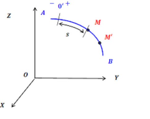
In this case, we will have to decide in which direction along the curve the coordinate s is measured in the positive direction and then the function

$$

$$s = s (t)$$

is also the law of motion. This method is convenient when we know the exact shape of the trajectory of a point.

3. Speed ​​and acceleration

Point speed is the first derivative radius of a point vector over time.

$$

$$\ vec v = \ frac {d \ vec r} {dt}$$

The velocity vector is tangential to the trajectory of the point.

Which, from many points of view, is the most correct and complete definition. If the motion of a point is defined by the coordinate method, then the velocity vector is determined by its projections on the coordinate axes, calculated as derivatives of the corresponding coordinates

$$

$$\ begin {cases} & v_x = \ cfrac {dx} {dt} = \ dot x \\ & v_y = \ cfrac {dy} {dt} = \ dot y \\ & v_z = \ cfrac {dz} {dt} = \ dot z \ end {cases}$$

The last designation of the derivative is a point over a function, as ancient as the Beginnings ... themselves and goes back to Newton. It was he who proposed this designation. Then the habitual for schoolchildren and students rooted as a symbol of a derivative with respect to an arbitrary parameter, and the dot remained as a symbol of a derivative taken precisely in time.

Point acceleration is the first derivative of the velocity vector of a point, or the second derivative of the radius vector of a point

$$

$$\ vec a = \ frac {d \ vec v} {dt} = \ frac {d ^ 2 \ vec r} {dt ^ 2}$$

In Cartesian coordinates it looks like this.

$$

$$\ begin {cases} & a_x = \ dot v_x = \ ddot x \\ & a_y = \ dot v_y = \ ddot y \\ & a_z = \ dot v_x = \ ddot z \ end {cases}$$

Here, two points above the functions denote the second time derivative.

Thus, knowing the law of motion of a point, we can easily determine its speed and acceleration by simple calculation of the derivative.

4. Dynamics axioms

The school talk about the laws of Newton. At the same time, they often make a fundamental mistake - they forget to say that these laws are formulated and are valid only for the material point. And they do not work at all for a solid (quieter, quieter, no angry cries, I will explain everything).

In such a scientific discipline as theoretical mechanics, Newton's laws are usually called axioms, and supplemented by the principle of independence of the action of forces, they form a system of dynamics axioms.

Axiom 1 (Newton's First Law)

A point moves in space uniformly and rectilinearly, if the vector sum of the forces applied to it is zero.

As a teacher of mechanics with quite good experience, I prefer this very formulation of the principle of inertia of classical mechanics than the confused school “there are such reference systems as to which blah blah blah ...”. From this formulation, it is immediately clear: for a mechanical movement to take place, it is not at all necessary an action of force. If there are no forces, or their action on a point is compensated, then its movement will occur by inertia, in a straight line with constant speed. For the direction and magnitude of the speed to change, you need a reason, namely

Axiom 2 (Newton's Second Law)

The acceleration vector of a point multiplied by its mass is equal to the force acting on a point.

$$

$$\ vec F = m \, \ vec a$$

If a non-zero force acts on a point, then it generates an acceleration directed in the same direction. And with the advent of acceleration, the speed of the point also changes, and hence the nature of the movement.

Axiom 3 (Newton's Third Law)

Two points interact with forces of equal magnitude, opposite in direction and directed along one straight line.

$$

$$\ vec F_ {1,2} = - \ vec F_ {2,1}$$

The fundamental nature of this law can not be overestimated, but its deep meaning can be understood by examples about which we will not talk now. So far, I propose to delve into the memory and re-read the school textbook. The following is much more important to us.

Axiom 4 (Principle of independence of action of forces)

If there are several forces acting on a point, the acceleration imparted by the point by these forces is equal to the geometric sum of the accelerations imparted to the point by each force separately.

From this it follows that when acting on a point of several forces, the equation

$$

$$m \, \ vec a = \ sum \ vec F_k$$

which in mechanics I call a proud and scary name is the differential equation of motion of a point in a vector form.

It is this equation that serves as the starting point for mathematical modeling in mechanics. Solving this particular equation, we will begin to master the basics of mathematical modeling as an independent scientific branch. Look at it attentively, rummage memory, open textbooks. We will remember him more than once.

Now I will explain what I meant by saying that Newton's laws are valid only for the material point. This is true, imagine a solid body moving in space. Damn it, go outside, pick up a bigger stick from the ground and throw it away. Do you see? Each point of the stick moves along its trajectory. So each point of the stick has its own acceleration . To which of these points does Newton's second law apply? It applies to every point of the stick, but not to the stick as a whole. The concepts "stick acceleration", "stick path" are meaningless. Acceleration and the trajectory of a particular point of the stick, for example, its center of mass, make sense.

That is why, when describing the motion of a solid body, one uses the dynamics theorems for a solid body: the theorem on the motion of the center of mass, the theorem on the change of the angular momentum and the theorem on the change in kinetic energy. Yes, these theorems are derived based on the axioms listed above (Newton's laws). But these laws are not directly applicable to the description of the motion of a rigid body. Only for point.

5. Differential equations of point motion

So, Newton's second law and the principle of independence of the action of forces give us a serious mathematical apparatus in the form of an equation that connects the acceleration point and the forces acting on this point. If we replace the acceleration, as defined above, by the second time derivative of the radius vector of a point, we will see the following expression

$$

$$m \, \ frac {d ^ 2 \ vec r} {dt ^ 2} = \ sum \ vec F_k$$

It seems to be simple, but in fact it is extremely cool and important. Look - on our left, there is a law of motion (yes, differentiated twice). And on the right - the sum of the forces. Thus, this equation connects the forces applied to a point and the law of motion. So, knowing the law of motion, one can calculate the force causing it. Or vice versa, knowing the forces applied to a point, find the law of motion.

In the overwhelming majority of cases, this equation is not used directly, but is laid out on three equations in projections on the coordinate axes.

$$

$$\ begin {cases} & m \, \ ddot x = \ sum F_ {kx} \\ & m \, \ ddot y = \ sum F_ {ky} \\ & m \, \ ddot z = \ sum F_ {kz} \ end {cases}$$

6. Tasks of point dynamics

Using the differential equations of motion, points solve two fundamental problems.

The first (inverse) task dynamics

According to the known law of motion of a point, determine the force acting on a point.

Suppose we know the law of motion of a point, given in the form of the dependence of the radius vector on time

$$

$$\ vec r = \ vec r (t)$$

Then, it is enough to take the time derivative of this function twice, multiply the result by the mass, and we will get the force that causes the point to move according to this law

$$

$$\ vec R = m \, \ frac {d ^ 2 \ vec r} {dt ^ 2}$$

I note that the resulting force is in fact the resultant of all forces applied to a point, that is, information about the force factors determining movement is incomplete. But, however, this principle allowed Newton to discover the law of world wideness. Nowadays, this problem has been generalized to arbitrary dynamic systems that are completely unrelated to mechanics and is known in control theory as a method of inverse problems of dynamics.

The second (direct) task dynamics

According to the known forces applied to the point, determine the law of its movement.

The forces applied to the point can be folded, resulting in a resultant vector. Moreover, this resultant in the general case will depend on time, the position of a point in space and its speed.

$$

$$m \, \ frac {d ^ 2 \ vec r} {dt ^ 2} = \ vec R \ left (t, \ vec r, \ frac {d \ vec r} {dt} \ right)$$

We have obtained an equation containing an unknown function. $$$\ vec r (t)$as well as its two derivatives. Such an equation in mathematics is called differential. Its solution ultimately boils down to integration — the operation of inversely finding the derivative. Since the equation contains the second derivative of the unknown function, it is a second-order equation, which means it will have to take the integral twice.

The search for integral in orders is more complicated than the search for derivative. And in most cases the result cannot be expressed in terms of elementary mathematical functions. As our teacher of mathematics at the university said: “If you see a bull, you can imagine what cutlets it is made of. But seeing the cutlets, you will never be able to reconstruct the bull according to them ... ”. In my opinion, this bike perfectly reflects the meaning and complexity of reverse operations.

The impossibility of obtaining an analytical solution of many problems led to the emergence of numerical methods, the rapid growth of which occurred in the computer age. On the day when the differential equation of motion was first solved on a computer, it was the birthday of a new branch of knowledge - mathematical modeling.

Conclusion

No need to blame me for reprinting a textbook on mechanics. This text is copyright and aims to review the theoretical foundations, without which talking about modeling as a practical field makes no sense. Next time we will practice, but we will begin as it should be from the beginning.

Thank you for your attention and see you soon!