What Robotics Can Teach Game AI
I am a robotics researcher and at the same time my hobby is game development. My specialization is the planning of multidimensional motion of robot manipulators. Traffic planning is a very important topic for game developers, it comes in handy every time you need to move a controlled AI character from one point to another.
In the process of studying game development, I found many tutorials telling about motion planning (usually in the game development literature it is called “finding the way”), but most of them didn’t go into details of what movement planning is from a theoretical point of view . As far as I can tell, in most games, some other motion planning is rarely used, except for one of the three serious algorithms: search on A * grids, visibility graphs and flow fields. In addition to these three principles, there is a whole world of theoretical studies of motion planning, and some of them may be useful to game developers.
In this article I would like to talk about the standard techniques of traffic planning in my context and explain their advantages and disadvantages. I also want to introduce the basic techniques that are not commonly used in video games. I hope they shed light on how they can be used in game development.
Movement from point A to point B: agents and targets
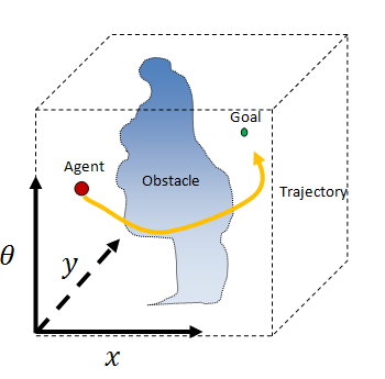
Let's start with the fact that we have an AI-controlled character in the game, for example, an enemy in a shooter or a unit in a strategic game. We will call this character an agent. The agent is located in a specific place in the world called its “configuration”. In two dimensions, the agent configuration can be represented by only two numbers (usually x and y). The agent wants to get to some other place in the world, which we will call the goal (Goal).
')
Let's imagine an agent in the form of a circle living in a flat two-dimensional world. Suppose that an agent can move in any direction he needs. If there is nothing but empty space between the agent and its target, the agent can simply move in a straight line from its current configuration to the target. When he reaches the goal, he stops. We can call this the “Walk To Algorithm”.
: WALK TO:.
: .

If the world is completely empty, then it fits perfectly. It may seem obvious that we need to move from the initial configuration to the configuration of the target, but it is worth considering that the agent could move in a completely different way to get from the current configuration to the target. He could cycle around until he reached the goal or move fifty kilometers away from it before returning and staying on the target.
So why do we think the straight line is obvious? Because in a sense, this is the “best” way of movement. If we accept that the agent can only move at a constant speed in any direction, then the straight line is the shortest and fastest way to get from one point to another. In this sense, the Walk To algorithm is optimal . In this article we will talk a lot about optimality. In essence, when we speak of the optimality of an algorithm, we mean that it is “better than everyone” with a certain criterion of “best”. If you want to get from point A to point B as quickly as possible and there is nothing on the way, then nothing compares to a straight line.
And in fact, in many games (I would say, even in most games), the algorithm for moving along a straight Walk To is ideal for solving a problem. If you have small 2D-enemies in the corridors or rooms that do not need to wander through the maze or follow the orders of the player, then you will never need anything more complicated.
But if something suddenly appeared on the way?

In this case, an object in the path (called an obstacle (Obstacle)) blocks the path of the agent to the target. Since the agent can no longer move directly to the goal, he simply stops. What happened here?
Although the Walk To algorithm is optimal , it is not complete . "Full" algorithm is able to solve all the problems in its field in a finite time. In our case, an area is circles moving in a plane with obstacles. Obviously, a simple move directly to the goal does not solve all the problems in this area.
To solve all the problems in this area and solve them optimally, we need something more sophisticated.
Reactive planning: beetle algorithm
What would we do if there were obstacles? When we need to get to the goal (for example, to the door), and there is something on the way (for example, a chair), then we just go around it and continue to move towards the goal. This type of behavior is called "avoiding obstacles." This principle can be used to solve our problem of moving the agent to the goal.
One of the simplest obstacle avoidance algorithms is the bug algorithm . It works as follows:
: BUG. M-.M- :, ., , M-, , M-. M-, 2.
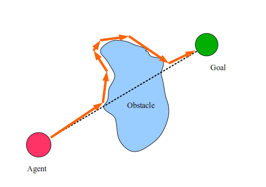
Step 2.2 requires an explanation. In fact, the agent remembers all cases of meeting with the M-line for the current obstacle, and leaves the obstacle only on the M-line and closer to the target than at any other time before. This is to avoid getting the agent into an infinite loop.
In the figure above, the dotted line shows the M-line, and the orange arrows indicate the steps taken by our agent to achieve the goal. They are called agent trajectories . Surprisingly, the beetle's algorithm is very easy to solve many problems of this type. Try to draw a bunch of crazy figures and see how well it works! But does the bug algorithm work for each task? And why does it work?
The simple beetle algorithm has a lot of interesting features and demonstrates many key concepts to which we will again return in this article. These concepts are: trajectory, politics, heuristics, completeness and optimality.
We have already mentioned the concept of a trajectory , which is a simple sequence of configurations or movements made by an agent in its path. The beetle algorithm can be considered a trajectory planner (Trajectory Planner), that is, an algorithm that obtains the initial configuration and the configuration of the target and returns the trajectory from the beginning to the target. (In the game development literature, it is also sometimes called the “path planner”).
But we must also mention the concept of politics . If we do not interpret the beetle’s algorithm as returning the full trajectory from the beginning to the target, but interpret it as sending the agent a set of instructions that allow you to reach the target from any point, simply using your own configuration as a guide, then the beetle’s algorithm can be called a control policy (Control Policy). A management policy is simply a set of rules that, based on the state of the agent, determines what actions the agent must perform next.
In the beetle's algorithm, the M-line is a clear indicator of where the agent should be located next. Why did we choose to follow the M-line, and not, say, a line from the current position of the agent to the target? The answer is that the M-line is just a heuristic . A heuristic is a general rule used to report the next step of the algorithm. This rule gives some human knowledge of the algorithm. Choosing a heuristic is often an important part of developing such an algorithm. When choosing the wrong heuristics, the algorithm may be completely inoperable.
Believe it or not (I didn’t believe at first), but the beetle's algorithm solves all the tasks in the field of two-dimensional circles, moving from the beginning to the goal. This means that regardless of the location of the agent or the goal, if the agent can achieve the goal, the bug’s algorithm will allow it to do so. Proof of this is beyond the scope of this article, but you can read about it if you wish. If an algorithm can solve all the problems in its field for which there are solutions, then it is called a complete algorithm .
But despite the fact that the beetle's algorithm can solve all the problems of this type, the trajectories it creates are not always the best possible categories by which the agent can achieve the goal. In fact, a bug’s algorithm can sometimes make an agent do pretty stupid things (just try to create an obstacle, small in a clockwise direction and huge in another direction, and you will understand what I mean. If we define “best” as “taking the shortest time, then the beetle's algorithm is by no means optimal .
Optimal planning: visibility graph
And if we need to solve the problem of moving circles among the obstacles along the optimal (shortest) path? To do this, we can involve the geometry in order to estimate what the optimal algorithm for solving this problem should be. First, note the following:
- On two-dimensional Euclidean planes, the shortest path between two points is a straight line.
- The length of a sequence of straight-line trajectories is the sum of the lengths of each of the lines.
- Since a polygon consists of straight lines (or edges), the shortest path that completely circumvents a convex polygon contains all the edges of the polygon.
- To bypass a nonconvex polygon, the shortest path contains all edges of the convex hull of the polygon.
- A point that is exactly on the edge of a polygon touches this polygon.
Understanding the definitions of "convexity", "nonconvexity" and "convex hull" is not very important for understanding this article, but these definitions are enough to create an optimal trajectory planner. Let's make the following assumptions:
- Our agent is a two-dimensional point of infinitely small size.
- All the obstacles of the world can be reduced to closed polygons .
- Our agent can move in any direction in a straight line.
Then we can find the optimal plan for the agent to achieve the goal by creating what is called the world visibility graph . In addition to geometry, we also need to know a little about the graphs. Graph theory is not the topic of this article, but in essence graphs are simply groups of abstract objects (called nodes ) connected to other nodes by abstract objects called edges . We can use the power of graphs to describe the world in which the agent lives. We can say that a node is any place where an agent can be, without touching anything. An edge is a path between nodes, along which an agent can move.
Taking this into account, we can define the visibility graph scheduler as follows:
: VISIBILITY GRAPH PLANNERG.G.G..G .V :V . , G.V. , G.(, A*) , .
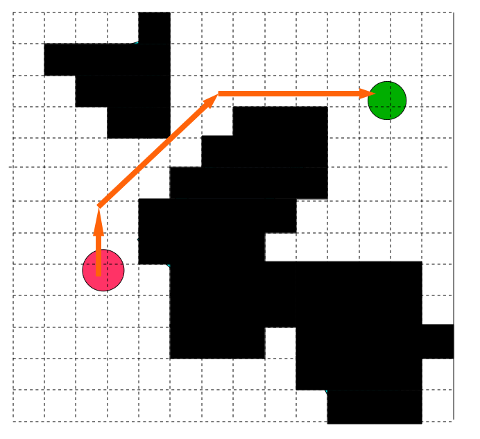
The visibility graph is as follows: (dashed lines)

And the final path looks like this:
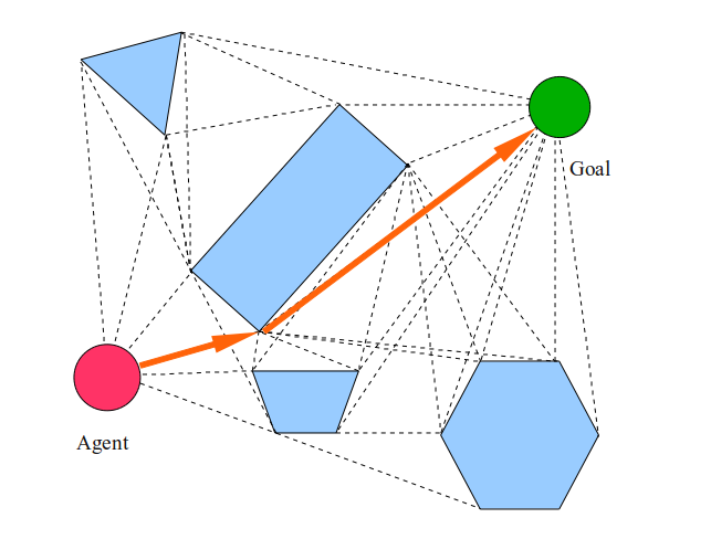
Because of the assumptions that an agent is an infinitely small point that can move along straight lines from any one location to any other, we have a trajectory that passes smoothly through corners, faces, and free space, which minimizes the distance goals
But what if our agent is not a point? Notice how the orange path leads the agent between the trapezoid and the rectangle. Obviously, the agent will not be able to squeeze through this space, so we need to solve this problem in some other way.
One solution is to assume that the agent is not a point, but a disk. In this case, we can simply inflate all obstacles to the agent’s radius, and then plan as if the agent is a point in this new bloated world.
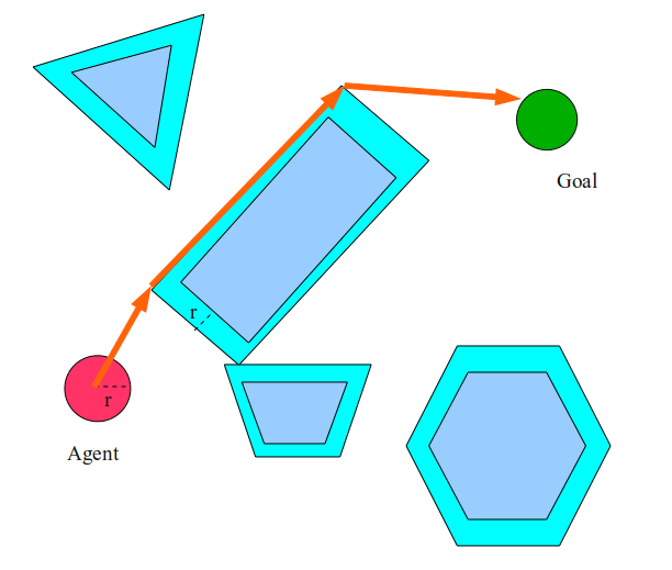
In this case, the agent will choose the path to the left and not to the right of the rectangle, because he simply does not fit in the space between the trapezoid and the rectangle. This inflating operation is in fact incredibly important. In essence, we changed the world so that our assumption that the agent is a point remains true.
This operation is called the calculation of the configuration space of the world. Configuration space (or C-Space) is a coordinate system in which the configuration of our agent is represented by one point. An obstacle in the workspace is transformed into an obstacle in the configuration space by placing the agent in the conditioned configuration and checking agent collisions. If in this configuration the agent touches an obstacle in the workspace, then it becomes an obstacle in the configuration space. If we have a non-circular agent, then we use the so-called sum for inflating obstacles.
Minkowski .
In the case of two-dimensional space, this may seem boring, but this is exactly what we are doing to “inflate” the obstacles. The new “inflated” space is actually a configuration space. In more multidimensional spaces, things get more complicated!
The visibility graph scheduler is a great thing. It is both optimal and complete , besides, it does not rely on any heuristics . Another great advantage of the visibility graph scheduler is its moderate multi-query capability. The multi-query scheduler can reuse old computations when working with new goals. In the case of a visibility graph, if the location of the target or agent changes, it is enough for us to just rebuild the edges of the graph from the agent and from the target. These benefits make this scheduler extremely attractive to game programmers.
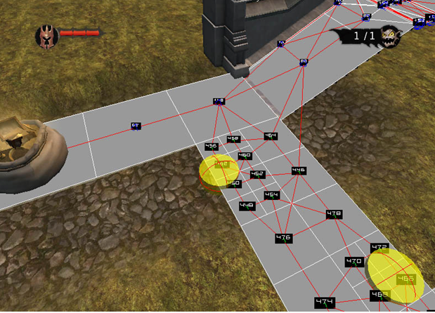
In fact, in many modern games, visibility graphs are used for planning. A popular variation of the visibility graph principle is the Nav (igation) Mesh . In Nav Mesh, visibility graphs are sometimes used as a basis (along with other heuristics for the distance to enemies, objects, etc.). Nav Mesh can be changed by designers or programmers. Each Nav Mesh is stored as a file and is used for each individual level.
Here is a screenshot of the Nav Mesh used in the Overlord video game:
Despite all its advantages, the methods of visibility graphs have significant drawbacks. For example, calculating the visibility graph can be quite a costly operation. With the increase in the number of obstacles, the size of the visibility graph increases significantly. The cost of calculating the visibility graph increases as a square of the number of vertices. In addition, when changing any obstacles, in order to maintain optimality, it is likely that a full recalculation of the visibility graph will be required.
Game programmers invented all sorts of tricks to speed up the creation of graphs using heuristics for selecting nodes to which you want to try to join through the edges. Also, game designers can give hints to the visibility graph algorithm so that it determines which nodes to connect in the first place. All these tricks lead to the fact that the graph of visibility ceases to be optimal and sometimes requires the monotonous work of programmers.
However, the most serious problem of visibility graphs (in my opinion) is that they do not generalize well. They solve one problem (planning on a 2D-plane with polygon obstacles), and solve it incredibly well. But what if we're not on a two-dimensional plane? What if our agent cannot be represented as a circle? What if we do not know what the obstacles will be, or they cannot be represented as polygons? Then we cannot, without tricks, use visibility graphs to solve our problem.
Fortunately, there are other methods that are closer to the “started and forgotten” principle, which solve some of these problems.
Lattice search: A * and its variations
Graphs of visibility work because they use the optimizing qualities of searching in abstract graphs, as well as the fundamental rules of Euclidean geometry . Euclidean geometry gives us a “fundamentally correct” search graph. And the abstract search itself is engaged in optimization.
But what if we completely abandon Euclidean geometry and simply solve the entire problem by searching through abstract graphs? In this way, we can eliminate the middleman in the face of geometry and solve many different types of problems.
The problem is that we can use a variety of different approaches to transfer our task to the search area by graphs. What will be the nodes? What exactly is considered ribs? What does connecting one node with another mean? How we answer these questions largely determines the performance of our algorithm.
Even if the graph search algorithm gives us the “optimal” answer, it is “optimal” in terms of only its own internal structure. This does not mean that the “optimal” according to the graph search algorithm the answer is the answer we need.
Given this, let's define the graph in the most common way: as a lattice . Here's how it works:
: DISCRETIZE SPACE, ., ., , ., , , ...
“Contiguous” is another aspect that needs to be attentive. Most often, it is defined as " any cell that has at least one common angle with the current cell " (this is called "Euclidean adjacency") or as " any cell that has at least one common edge with the current cell " (this is called "Manhattan adjacency" ). The choice of the definition of adjacency greatly depends on the answer returned by the graph search algorithm.
Here is what the sampling stage will look like in our case study:
If we search for this column according to the Euclidean adjacency metric, we get something like this:
There are many other graph search algorithms that can be used to solve the grid search problem, but the most popular is A * . A * is related to Dijkstra’s algorithm , which performs a search on nodes using heuristics, starting with the starting node. A * is well researched in many other articles and tutorials, so I will not explain it here.
A * and other grid graph search methods are one of the most common scheduling algorithms in games, and a discretized grid is one of the most popular ways to structure A *. For many games, this search method is ideal, because many games still use tiles or voxels to represent the world.
The search methods for graphs on a discrete lattice (including A *) are optimal according to their internal structure. They are also resolution-complete . This is a weaker form of completeness, which states that when the fineness of the lattice tends to infinity (that is, when the cells tend to an infinitely small size), the algorithm solves more and more problems to be solved.
In our particular example, the grid search method is single-request , and not multi- request , because the search by column usually cannot reuse old information when generalizing to the new configurations of the goal and the beginning. However, the sampling stage, of course, can be reused.
Another key advantage (in my opinion, mainly) of graph-based methods is that they are completely abstract.This means that additional costs (such as ensuring security, smoothness, proximity of necessary objects, etc.) can be automatically taken into account and automated. In addition, to solve completely different problems, you can use the same abstract code. In the DwarfCorp game , we use one A * scheduler for both motion planning and symbolic action planning. (used to represent actions that agents can perform as an abstract graph).
However, a grid search has at least one serious drawback: it is incredibly demanding of memory. If each node is built in a naive way from the beginning, then with an increase in the size of the world, your memory will end very quickly. Most of the problem lies in the fact that the grate must keep large volumes of empty space. To minimize this problem, there are optimization techniques, but in fundamental terms, as the size of the world increases and the number of measurements of the task increases, the memory size in the grid increases monstrously. Therefore, this method is not applicable to many more complex tasks.
Another serious disadvantage of the method is that the search in the columns by itself can take quite a long time. If there are several thousand agents moving in the world at the same time or a multitude of obstacles changing their position, then a search in a grid may be inapplicable. In our game DwarfCorp, several streams are devoted to planning. It eats away a bunch of CPU time. In your case, this can also be!
Management Policies: Potential Functions and Flow Fields
Another way to solve the task of planning a movement is to stop thinking about it in the categories of planning trajectories and begin to perceive it in categories by management policy . Remember, we said that the beetle algorithm can be perceived as both a trajectory planner and a control policy? In that paragraph, we defined a policy as a set of rules that takes a configuration and returns an action (or “control input”).
The beetle's algorithm can be perceived as a simple control policy, which simply tells the agent to move towards the target until he stumbles upon an obstacle, and then bypass the obstacle in a clockwise direction. The agent can literally follow these rules, moving along its path to the goal.
The key advantages of management policies are that they generally do not rely on an agent who has something more than local knowledge of the world and that they are incredibly fast in calculations. Thousands (or millions) of agents can easily follow the same management policy.
Can we think of any management policies that work better than the beetle's algorithm? It is worth considering one of them, a very useful " potential field policy ". It simulates an agent in the form of a charged particle, attracted to the target and repelled by obstacles:
: POTENTIAL FIELD POLICYa bg.o.o r.u = a * g^ + B * r^, v^ v..
Understanding this policy requires some knowledge of linear algebra . In essence, the control input is a weighted sum of two members: a member of attraction and a member of repulsion . The choice of weights in each member significantly affects the final trajectory of the agent.

With the help of a potential field policy, agents can be made to move in an incredibly realistic and smooth manner. You can also easily add additional conditions (proximity to the desired object or the distance to the enemy).
Since the policy of a potential field is extremely quickly calculated in parallel computing, this method can very effectively control thousands and thousands of agents. Sometimes this control policy is calculated in advance and stored in the grid for each level, after which it can be changed by the designer in the way he needs (then it is usually called the flow field ).
In some games (especially strategic ones) this method is used with great efficiency. Here is an example of flow fields used in a strategy game.Supreme Commander 2 , so that units naturally avoid each other, keeping the build:
Of course, the functions of the flow fields and the potential fields have serious drawbacks. First, they are by no means optimal . Agents will be distributed by the flow field regardless of how long it takes to get to the goal. Secondly (and, in my opinion, this is the most important), they are by no means complete . What if the control input is reset before the agent reaches the target? In this case, we will say that the agent has reached a " local minimum ". You may think that such cases are quite rare, but in fact they are quite easy to construct. Simply place a large U-shaped obstacle in front of the agent.
Finally, flow fields and other control policies are very difficult to configure. How do we choose the weight of each member? In the end, they require manual tuning to get good results.
Typically, designers have to manually adjust the flow fields to avoid local minima. Such problems limit the possible utility in the general case of flow fields. However, in many cases they are helpful.
Configuration Space and Curse of Dimension
So, we discussed the three most popular motion-planning algorithms in video games: gratings, visibility graphs, and flow fields. These algorithms are extremely useful, simple to implement, and have been well studied. They work ideally in the case of two-dimensional problems with circular agents moving in all directions of the plane. Fortunately, almost all tasks in video games are related to this case, and the rest can be imitated with cunning tricks and designer hard work. It is not surprising that they are so actively used in the gaming industry.
And what did the movement planning researchers have been doing for the last few decades? Everyone else. What if your agent is not a circle? What if he is not on a plane? What if he can move in any direction? What if goals or obstacles are constantly changing? Answering these questions is not easy.
Let's start with a very simple case, which seems to be quite simple to solve with the help of the methods we have already described, but which is actually impossible to solve with these methods without fundamentally changing them.
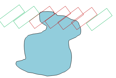
What if the agent is not a circle but a rectangle? What if an agent's turn is important ? Here is what the picture I am describing looks like:

In the case shown above, the agent (red) looks like a shopping cart, which can move in any direction. We want to move the agent so that it is exactly on top of the target and turned in the right direction.
Here we can presumably use the beetle's algorithm, but we will need to carefully handle the turns of the agent so that it does not encounter obstacles. We will quickly become entangled in the chaos of rules that are not quite as elegant as for the case of a round agent.
And what if you try to use the graph of visibility? To do this, the agent must be a point. Remember how we did the trick and inflated the objects for the round agent? Perhaps in this case it will be possible to do something similar. But how much do we need to inflate objects?
A simple solution would be to choose the “worst case scenario” and calculate the planning with this calculation. In this case, we simply take the agent, determine the circle that describes it, and accept the agent as an equal circle of this size. Then we inflate the obstacles to the desired size.

It will work, but we will have to sacrifice fullness. There will be many tasks that we can not solve. Take, for example, such a task, in which a long and thin agent must, in order to achieve a goal, sneak through a “keyhole”:

In this scenario, the agent can reach the target, penetrate the well, rotate 90 degrees, then reach the next well, rotate 90 degrees and exit. With a conservative approximation of the agent through the circle that describes this problem it will be impossible to solve.
The problem is that we have not correctly taken into account the configuration space of the agent. Up to this point, we have been discussing only 2D planning in the environment of 2D obstacles. In such cases, the configuration space is well transformed from two-dimensional obstacles to another two-dimensional plane and we observe the effect of “inflating” obstacles.
But in fact, the following happens here: we added another dimension to our planning task. The agent has not only a position in x and y, but also a rotation. Our task is actually a three-dimensional planning task. Now the transformations between working and configuration spaces are becoming much more complex.
You can take it as follows: Imagine that the agent performed a certain turn (which we denote theta). Now we move the agent to each point of the workspace with a given rotation, and if the agent touches an obstacle, then we consider this point to be a collision in the configuration space. Such operations for polygon obstacles can also be implemented using Minkowski sums .
In the diagram above, we have one agent passing through an obstacle. Red contours of the agent show configurations that are in collision, and green contours show configurations without collisions. This naturally leads to another “swelling” of obstacles. If we execute it for all possible positions (x, y) of the agent, then we will create a two-dimensional cut of the configuration space.
Now we will simply increase the amount of the aunt and repeat the operation, receiving another two-dimensional slice.

Now we can put the cuts one on another, aligning their x and y coordinates, as if folded sheets of graph paper:

If we cut the aunt infinitely thin, as a result we get the three-dimensional configuration space of the agent. This is a continuous cube, and theta is turned around from bottom to top. Obstacles turn into strange cylindrical shapes. The agent and his goals become just points in this new strange space.
It is quite difficult to put in my head, but in a sense, this approach is beautiful and elegant. If we can imagine obstacles in two dimensions, where each dimension is simply the position of the agent in x and y coordinates, then we can also represent obstacles in three dimensions, where the third dimension is the rotation of the agent.
What if we wanted to add another degree of freedom to the agent? Suppose we would like to increase or decrease its length? Or would he have arms and legs that also need to be considered? In such cases, we do the same thing - just add dimensions to the configuration space. At this stage, it becomes completely impossible to visualize, and in order to understand them, you have to use such concepts as “hyperplane”, “diversity with constraints” and “hyperpersons”.
An example of a four-dimensional planning problem. The agent consists of two segments with the axis connecting them.
Now that our agent is just a point in 3D space, we can use ordinary algorithms to find the solution to any motion planning problem. If we wanted, we could create a grid of voxels in the new 3D space and use A *. If they thought, they could also find a representation of the configuration space in the form of a polygonal mesh, and then use the visibility graph in 3D.
Similarly, for other dimensions, we can do the following:
- Calculate the agent and obstacle configuration space.
- Run A * or Nav Mesh in this space.
Unfortunately, these operations have two huge problems:
- N- NP- .
- N- NP- .
The technical term from computer science " NP-complex " means that the task as it increases becomes exponentially more difficult, carrying with it many other theoretical difficulties.
In practice, this means that if we start adding measurements to planning tasks, we will very soon exhaust the computational power or memory, or both. This problem is known as the curse of dimension . In three dimensions, we can do with A *, but as soon as we get to 4, 5 or 6 dimensions, A * quickly becomes useless (despite recent research by Maxim Likhachev , which ensured his fairly good performance).
The simplest example of a six-dimensional scheduling problem is called "the task of moving the piano ". Its wording: how to move a solid object (say, a piano) from point A to point B in 3D-space, if it can be moved and rotated in any direction?

An example of the task of moving the piano from the OMPL.
Surprisingly, despite its simplicity, this task has remained unsolved for decades.
For this reason, the games basically adhere to simple two-dimensional tasks and imitate everything else (even when having a solution to something like the task of moving the piano seems like a fundamental part of the AI of a three-dimensional game).
Unresolved Tasks
In the 70s and 80s, motion planning studies focused on fast ways to calculate configuration space and good compression heuristics for reducing the dimension of some planning tasks. Unfortunately, these studies did not lead to the creation of simple common solutions to problems in a large number of dimensions. The situation did not change until the 90s and the beginning of zero years, when robotics researchers did not begin to move the progress of solving common multidimensional problems.
Today, planning in multidimensional spaces is much better studied. All this happened thanks to two major discoveries: randomized planners and fast optimizers of trajectories . I will talk about them in the following sections.
The difference between finding a way and planning a move
I noticed that after the publication of the draft of this article, some readers were confused by my terminology. In the game development literature, the action of moving from point A to point B is usually called " finding the path ", and I called it " motion planning ." In essence, motion planning is a generalization of a path search with a looser definition of a “point” and a “path” that takes into account spaces of higher dimension (for example, turns and hinges).
Traffic planning can be perceived as a search for a path in the agent's configuration space.
Randomized Planning: Probabilistic Road Maps, PRM
One of the first common solutions to multidimensional planning problems is called a probabilistic roadmap . It borrows the ideas of the Navigation Mesh and the visibility graph, adding another component: randomness.
To begin, I will present introductory information. We already know that the most difficult aspects of planning in multidimensional spaces consist in calculating the configuration space and further finding the optimal path through this space.
PRM solves both of these problems, completely rejecting the idea of computing configuration space and forgetting about the principle of optimality. With this approach, a visibility graph in space is randomly created using distance heuristics, and then a solution is searched for in this visibility graph. You can also make the assumption that we can relatively inexpensively perform a collision check of any agent configuration.
This is how the entire algorithm looks like:
: PROBABALISTIC ROAD MAP (PRM)GG .N :R. .R, ., R G.G, d R.N,R N, G.A* .

In short, at each stage we create a random point and connect it with the neighbors in the graph based on what neighbors of the graph it “sees”, that is, if we are sure that we can draw a straight line between any new node and neighbors in the graph .
We immediately see that this is very similar to the visibility graph algorithm, except that we never mention “for each obstacle” or “for each vertex”, because, of course, such calculations will be NP-complete.
Instead, PRM considers only the structure of the random graph created by it and collisions between neighboring nodes.
PRM Properties
We have already said that the algorithm is no longer optimal and is not complete. But what can we say about its performance?
PRM algorithm is so-called "probabilistically complete ". This means that when the number of iterations N goes to infinity, the probability that PRM solves any solvable scheduling request is equal to one. This seems to be a very shaky definition (it is), but in practice PRM converges to the correct solution very quickly However, this means that the algorithm will have a random speed and may hang forever without finding a solution.
PRM also has interesting relationships with optimality. As PRM increases in size (and N grows to infinity), the number of possible paths increases. ad infinitum, and the optimal path through PRM becomes the truly optimal path through configuration space.
As you can imagine, because of its randomness, PRM can create very ugly, long and dangerous ways. In this respect, PRM is by no means optimal.
Like Nav Mesh visibility graphs, in fundamental terms, PRM are multi-query schedulers. They allow the agent to reuse a random graph efficiently for multiple scheduling requests. Level designers can also “bake” one PRM for each level.
Why an accident?
The most important “trick” of PRM (and other randomized algorithms) is that it presents the configuration space statistically and not explicitly. This allows us to sacrifice the optimality of the decision for the sake of speed, making “good enough” decisions where they exist. This is an incredibly powerful tool, because it allows the programmer to decide how much work the planner must do before returning the solution. This property is called the real-time execution algorithm property .
In essence, the complexity of the PRM grows with an increase in the number of samples and the distance parameter d, and not with an increase in the number of dimensions of the configuration space. Compare this with A * or visibility graphs, which spend exponentially more time as the dimension of the task increases.
This property allows PRM to quickly perform scheduling in hundreds of dimensions.
Since the invention of PRM, many different variants of the algorithm have been proposed, increasing its efficiency, the quality of the laid path, and ease of use.
Randomized random study trees (Randomly Exploring Randomized Trees, RRT)
Sometimes PRM multi-request is not required. Quite often, it is preferable to just get from point A to point B, without knowing anything about previous scheduling requests. For example, if the environment between scheduling requests changes, it is often better to simply reschedule from scratch than to recreate stored information obtained from previous scheduling requests.
In such cases, we can change the idea of creating random graphs, given that we only want to plan the movement from point A to point B. Once. One of the ways to do this is to replace the graph with a tree.
A tree is simply a special type of graph in which nodes are ordered into “parent” and “children” so that each tree node has exactly one parent node and is from zero and more children.
Let's see how our traffic planning can be represented as a tree. Imagine if the agent systematically explores configuration space.
If the agent is in some state, then there are several other states in which he can go from the current (or, in our case, an infinite number of states). From each of these states he can go to other states (but will not go back because he was already in the state from which he came).
If we store the states in which the agent was, as “parent” nodes, and all the states to which the agent passes from them as “children”, then we can form a tree-like structure growing from the current state of the agent to all places, in which the agent may potentially be located. Sooner or later, the agent tree will direct it to the goal state and we will have a solution.
This idea is very similar to the A * algorithm, which systematically expands states and adds them to a tree-like structure (from a technical point of view, to a directed acyclic graph).
So can we randomly grow a tree from the initial configuration of the agent to achieve the configuration of the goal?
This task is sought to solve two classes of algorithms. Both were invented in the late 90s and early zero. One of the approaches is “nodocentric” - it selects a random node in the tree and grows in a random direction. This class of algorithms is called “EST”, that is, “Expansive Space Trees” (“expandable spatial trees”). The second approach is “sample-oriented”: it starts with a random sample of nodes in space, and then grows the closest node towards this random sample. Algorithms of this type are called " RRT " ("Rapidly Exploring Randomized Trees", "randomized random study trees").
In general, the RRT is much better than EST, but the explanation of the reasons for this are beyond the scope of this article.
This is how the RRT works:
: RAPIDLY EXPLORING RANDOMIZED TREE (RRT)T.T .N ,R.T R . K.K R , :.T .d K, .
d , .

The pictures above show approximately one step of the algorithm in the middle of its execution. We take a random sample (orange, r), find the node closest to it (black, k), and then add one or more new nodes that take a “step in the direction” of the random sample.
The tree will continue to grow so randomly until it reaches the goal. From time to time we will also perform random sampling to the target, in an eager manner trying to draw a straight line towards it. In practice, the probability of hitting a target in a sample will, at best, be in the range from 30% to 80%, depending on the clutter in the configuration space.
RRT is relatively simple. They can be implemented in just a few lines of code (assuming that we can easily find the closest node in the tree).
RRT properties
You probably will not be surprised that the RRT algorithm is only probabilistically complete . It is non-optimal (and in many cases excessively non-optimal).

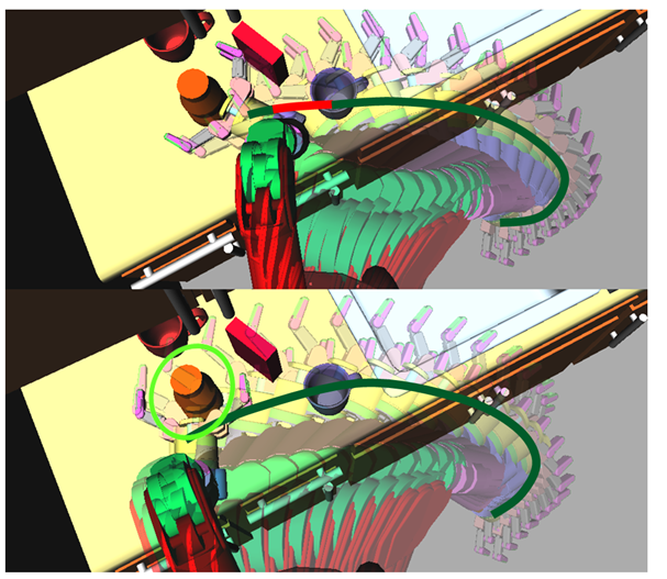
Robot manipulators are considered very multidimensional systems. In this case, we have two manipulators with seven hinges each, holding single-pliers. The system is 15-dimensional. Modern motion planning studies are studying similar multidimensional systems.
Due to its simplicity, RRT also usually turns out to be extremely fast (at least for multidimensional systems). When using the fastest variations, RRT solutions for seven-dimensional or more multi-dimensional systems are found in milliseconds. When the number of measurements reaches tens, RRT usually surpasses all other planners in solving such problems. But it is worth considering that “fast” in the community of researchers of multidimensional planning means a secondor so to perform the entire pipeline of actions in seven dimensions, or up to a minute with twenty or more measurements. The reason for this is that the RRT paths are often too terrible to use directly, and must go through a long preprocessing stage. This can shock programmers using A *, which returns solutions to two-dimensional problems in milliseconds; but try performing A * for a seven-dimensional task - it will never return a solution !
RRT Variations
After the invention of the RRT algorithm and the conquest of great success, many attempts were made to extend it to other areas or increase its performance. Here are some of the variations of RRT that you should know about:
RRTConnect- grows two trees from the beginning and from the target, and tries to connect them with a straight line at random intervals. As far as I know, this is the fastest scheduler for tasks with a high number of measurements. Here is a beautiful illustration of the RRT connect I created (white - obstacles, blue - free space):

RRT * - invented this decade. Ensures optimality through rebalancing the tree. Thousands of times slower than RRTConnect.
T-RRT - trying to create high-quality RRT-paths, exploring the gradient of the cost function.
Constrained RRT - allows you to perform planning with arbitrary restrictions (such as distance, cost, etc.). Slower than RRT, but not by much.
Kinodynamic RRT- performs planning in the space of input control signals, and not in the configuration space. Allows you to perform planning for cars, carts, ships and other agents who cannot arbitrarily change their turn. Actively used in the DARPA Grand Challenge. Much, much, much MUCHER slower than non-cynical dynamic planners.
Discrete RRT is an implementation of RRT for grids. In two-dimensional space, it is comparable in speed with A *, in 3D and in multidimensional systems, faster than it.
DARRT - invented in 2012. Implementing RRT for planning symbolic actions (previously considered to be the A * scope).
Path cutting and optimization
Since randomized planners do not guarantee optimality, the trajectories they create can be quite terrible. Therefore, instead of using them directly for agents, the random paths created by randomized planners are often passed on to complex optimization steps that increase their quality. Such optimization steps now take up most of the planning time for randomized planners. A seven-dimensional RRT may take a few milliseconds to return a possible path, but it may take up to five seconds to optimize the final path.
In the general case, the trajectory optimizer is an algorithm that obtains the original trajectory and the cost function, modifying the original trajectory so that it has the lowest cost. For example, if the cost function we need is to minimize the length of the trajectory, then the optimizer for this function will take the original trajectory and change this trajectory so that it is shorter. This type of optimizer is called a trajectory shortcutter .
One of the most common and extremely simple path cutters (which can be called the “stochastic climb climber”, Stochastic Hill Climbing Shortcutter) works as follows:
: Stochastic Hill Climbing ShortcutterN :T ( t1 t2)t1 t2 , ., t1 t2, T t1 t2,

This path cutter can be easily converted by replacing the concept of “short path” with any other cost function (for example, distance from obstacles, smoothness, safety, etc.). Over time, the trajectory will fall into what is called the “local minimum” of the cost function. The length (or cost) of the trajectory will no longer decrease.
There are more complex trajectory optimizers that work much faster than the climb I described. Such optimizers often use the knowledge about the scope of the planning task to speed up the work.
Optimization of the trajectory when planning
Another way to solve multidimensional motion planning problems is to step back from the idea of “finding space” to find a path, and instead focus directly on optimizing the trajectories.
If it is true that we can optimize the trajectory so that it is shorter or meets some other criterion, is it possible to solve the entire problem using optimization directly?
There are a large number of motion planners who use optimization to directly solve planning problems. Usually for this they represent the trajectory using a parametric model, and then intelligently change the parameters of the model until a local minimum is reached.
One of the ways to implement this process is called gradient descent.. If we have a certain cost function C (T) , where T is the trajectory, then we can calculate the gradient D_C (T) , which tells us how to change the given trajectory in such a way as to minimize costs.
In practice, this is a very difficult process. You can imagine it like this:
: Gradient Descent Trajectory Optimizer, .. T_0., , , ., - . , , 3.4., .
Over time, the trajectory will gradually “push off” from obstacles, nevertheless remaining smooth. In the general case, such a scheduler cannot be complete or optimal , because it uses the original straight line hypothesis as a strong heuristic. However, it can be locally complete and locally optimal (and in practice it solves most problems).

Note that in the image the gradients of the points are * negative * gradient of the cost function)
In practice, optimization of the trajectories as planning is a rather difficult and complicated topic that is difficult to judge in this article. What does trajectory gradient actually mean? What does perception of the trajectory as a rubber band mean? There are very difficult answers to these questions related to variation analysis.
We just need to know that the optimization of trajectories is a powerful alternative to randomized and search planners for multidimensional traffic planning. Their advantages are exceptional flexibility, theoretical guarantees of optimality, extremely high track quality and relative speed.
CHOMP, used by the robot for raising circles (Illustration from the work of Dragan et. Al )
In recent years, there have been many very fast trajectory optimizers that have become strong competitors of RRT and PRM in solving multidimensional problems. One of them, CHOMP , uses a gradient descent and a smart view of obstacles using the distance field. The other, TrajOpt , represents obstacles in the form of convex sets and uses techniques of sequential quadratic programming.
Important topics we didn't cover
In addition to what I have said, there is still a whole world of theoretical movement planning. Briefly talk about what else is.
Nonholonomic planning
We considered only the case when an agent can move in any direction at any speed. But what if it is not? For example, a car cannot slide sideways, but must move forward and backward. Such cases are called “nonholonomic” planning tasks. There are several solutions to this problem, but none of them is fast! It can take up to a minute to calculate the average plan for a modern car scheduler .
Restricted Planning
Nonholonomic planning refers to another set of tasks called “planning tasks with constraints”. In addition to restrictions in movement, there may also be restrictions on the physical configuration of the agent, the maximum force applied by the agent to the movement, or areas in which the agent is limited to objects other than obstacles. In generalized constrained planning there are also many solutions, but only some of them are fast .
Time planning
We can add another dimension to our plans, so that agents can, for example, track a moving target or avoid moving obstacles. When properly implemented, such techniques can produce surprising results. However, this problem remains intractable, because the agent often cannot predict the future.
Hybrid planning
What if our agent’s plan cannot be represented by a single path? What if the agent should interact along the way with other objects (and not just avoid them)? These types of tasks are usually referred to as “hybrid planning” - usually there is some abstract aspect connected by a geometric aspect of the task. For these types of tasks there are also no clear, universally accepted decisions.
findings
In this article, we discussed some basic concepts of motion planning and presented several classes of algorithms that solve the problem of moving an agent from point A to point B, from the simplest to the extraordinarily complex.
Modern progress in traffic planning studies has led to the fact that a wide range of previously unsolvable problems can now be solved on personal computers (and potentially in video game engines).
Unfortunately, many of these algorithms are still too slow to be applied in real time, especially for cars, ships and other vehicles that cannot move in all directions. All this requires further research.
I hope the article did not seem too complicated to you and you found something useful for yourself in it!
Here is a summary table of all the algorithms discussed in the article (it is necessary to take into account that only non-dynamical planning is taken into account here):

Source: https://habr.com/ru/post/349044/
All Articles