Backblaze statistics, a scientific approach to analyzing drive reliability

The firm Backblaze regularly publishes statistics on the failures of its hard drives, and even laid out in free access the full archov with the SMART statistics of the parameters of all their drives.

In this article I will show how using with scrap and some mother using scientific methods to calculate the reliability of drives.

Survival Analysis

In statistics, a section called “survival analysis” deals with survival or reliability analysis .

In short, this is a set of methods that allow comparing and counting how various factors affect life expectancy (in medicine), time between failures (in mechanics), etc. In general, this is an analysis of the time before the onset of some event. That is, to answer the question, such as: “What will be the proportion of survivors among patients some time after the applied treatment technician?” Or “What percentage of accumulators will fail next year?”.

At the same time, the answers to such questions must be sought when the time of observation of the patients (or accumulators) is limited and it is not possible to determine the lifetime of all patients.

Terms

• “Event” - the death of the patient, the first failure, etc., the time to which we can or want to measure
• “Time” is actually the time from the beginning of the observation until the occurrence of the event, or until the moment when we are not able to continue the observation (the patient left, the drive was turned off, etc.)
• “Censoring” - stopping the observation of the patient before the occurrence of the “Event”. Not relevant to the system of state supervision over the content and dissemination of information.
• “Survival function” , usually denoted as S (t) - the probability that the patient lives to time t, it is usually assumed that S (0) = 100% and the function does not increase over time.
• The “risk function” (“Hazard function”) - h (t) is the probability that the patient will die at time t, per unit of time. That is, the first derivative of the survival function with a minus sign.

Data

Backblaze laid out in open access a database with all the SMART parameters of all its hard drives, in .csv format, divided into files by day. If all these files are imported into the database (they offer their own scripts for importing into sqlite3), then we get a table with 90126570 entries, it takes about 19 GB and describes 122619 drives. I made a small script that pulls the following data about each drive into one table: manufacturer, model, serial number, capacity, service start date, operation time either until the end of the observation (SMART 9 parameter), or before the event and an indication of the event. A CSV file with this information can be downloaded here :

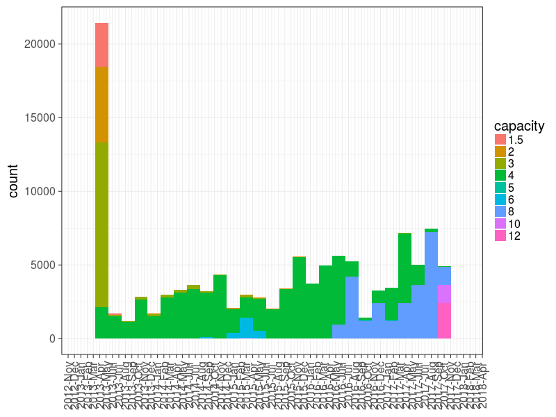
Schedule 0 : Distribution of drives by volume and date of commissioning.

Statistics

For processing, I will use R with tidyverse, survival, survminer, zoo packages
To begin with, an example of how to represent the function of survival:

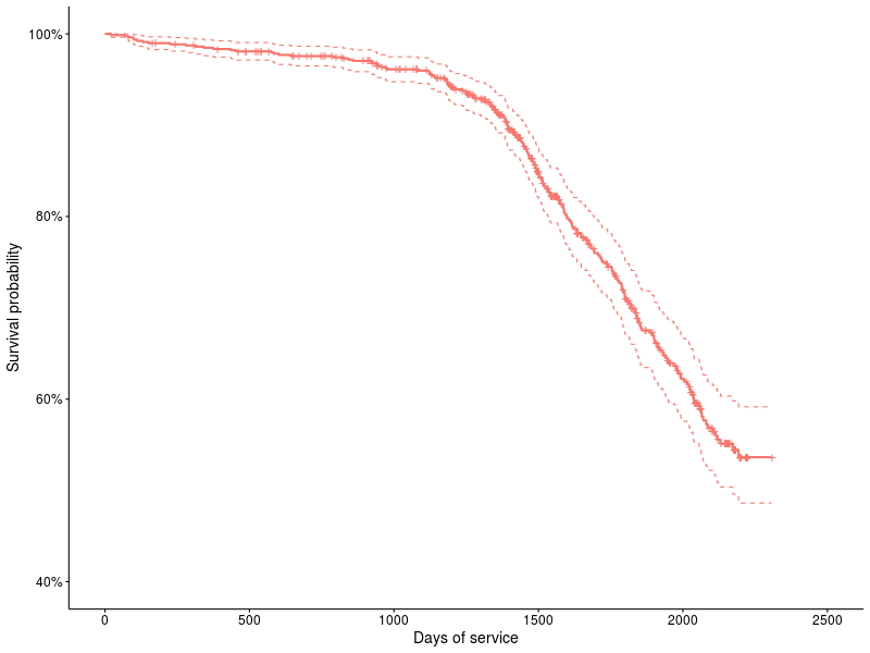
Graph 1 : The survival function for the ST31500341AS drive.

We look at schedule 1: This is an example of a survival schedule according to the Kaplan-Meier methodology, the percentages of surviving devices are plotted on the vertical axis, and the number of days on the horizontal axis. Crosses show censored devices (i.e., they have survived at least until X, and then traces are lost). Dotted lines indicate 95% confidence intervals. The Kaplan-Meier methodology ( KM ) appeared back in the year 58 and has since been actively used to describe the survival function, it should be noted that this is a non-parametric method, and uses a piecewise linear function to approximate the survival function (that is, with a small amount of data are clearly visible steps). In the survival package, this is done as follows:

 survfit(Surv(age_days, status) ~ 1, ...) 

Where as an argument first comes the formula where on the left a special function Surv shows that we are dealing with data and events, and then the data source: age_days - time, status - the code for the event (1 - events occurred, 0 - data rationalized). The result can be beautifully drawn using the survminer .

The KM method allows you to compare the survival functions with each other to determine if there is a statistically significant difference between them, for example, you took data on two drive models: ST31500341AS and ST31500541AS:

 survfit(Surv(age_days, status) ~ model, ...)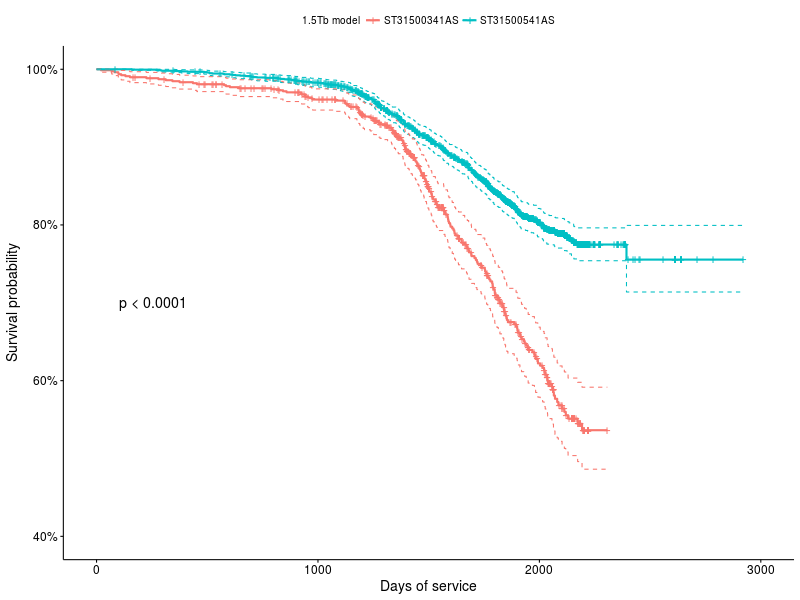 

Chart 2 : Survival functions for ST31500341AS and ST31500541AS drives

For comparison of distributions we use the survdiff function:

 survdiff(Surv(age_days, status) ~ model, ...) N Observed Expected (OE)^2/E (OE)^2/V model=ST31500341AS 787 216 125 66.4 84.3 model=ST31500541AS 2188 397 488 17.0 84.3 Chisq= 84.3 on 1 degrees of freedom, p= 0 

For us, the most important thing is the last line, with the value of p, it shows the probability that the distributions are not significantly different, in this case it is even evident that this cannot be.

It is worth noting that in this way you can only say - is there a difference or not, that is, it is not possible to say that strata A dies XX% faster than strata B.

Another interesting graph, let's see how the vitality of the most popular backblaze drive (ST4000DM000) changed with the installation time:

 survdiff(Surv(age_days, status) ~ start_quarter, ...)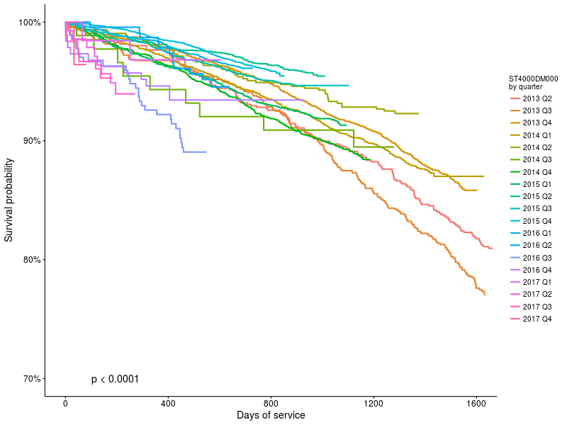 

Chart 3 : Survival functions for ST4000DM000 drives, depending on the start date.

It can be seen that there is a difference (p <0.0001) but it is interesting to know how big it is.

Cox proportional hazards model

And here Cox’s proportional risk model comes to our aid; it allows us to estimate the relative risks between different strata, but proceeds from the assumption that they all differ from each other in a strictly proportional manner.

For the calculation, the coxph function is used:

 model_coxph<-coxph(Surv(age_days, status) ~ make + capacity + year, ...)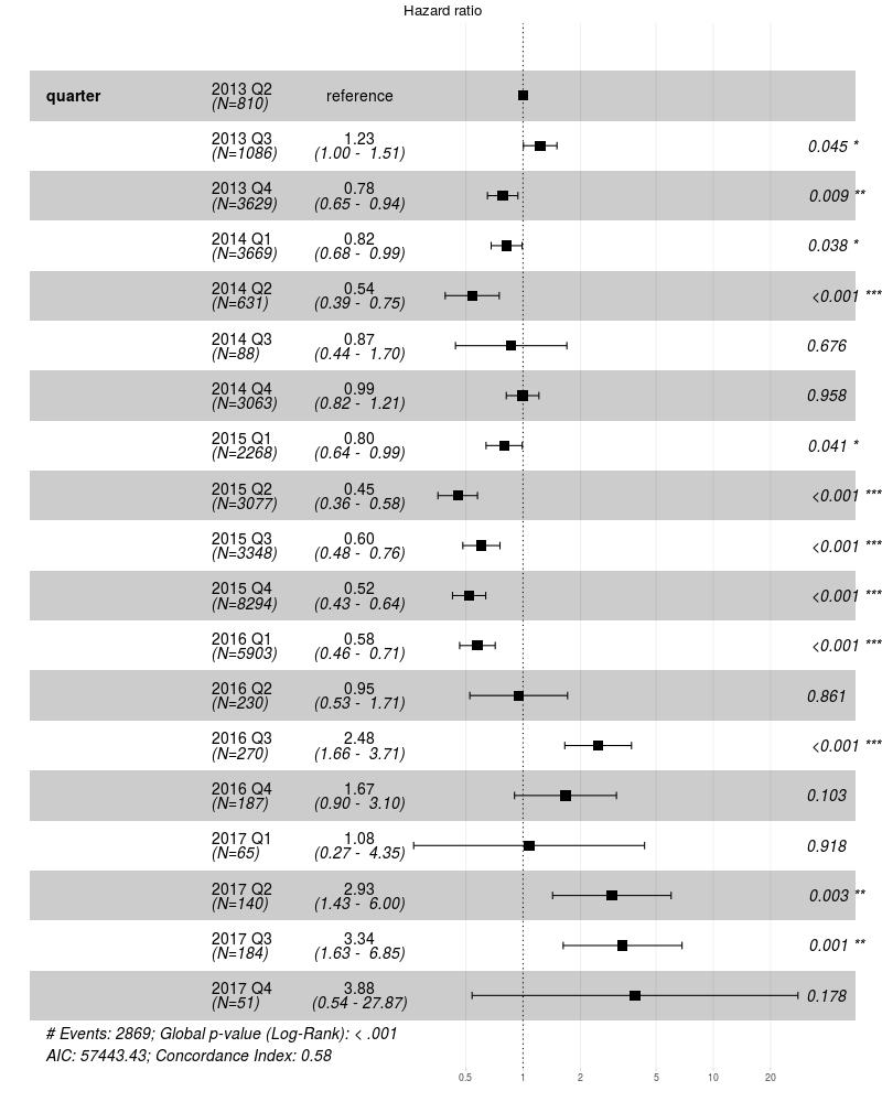 

Chart 4 : Relative risk factors (i.e. dying rate) for ST4000DM000 depending on the installation quarter. Asterisks show quarters when the speed of dying differs significantly from the base (in the first quarter of 2013).

Now let's compare the 4 most popular models of large drives: 8Tb: ST8000NM0055, ST8000DM002 10Tb ST10000NM0086 and 12Tb ST12000NM0007

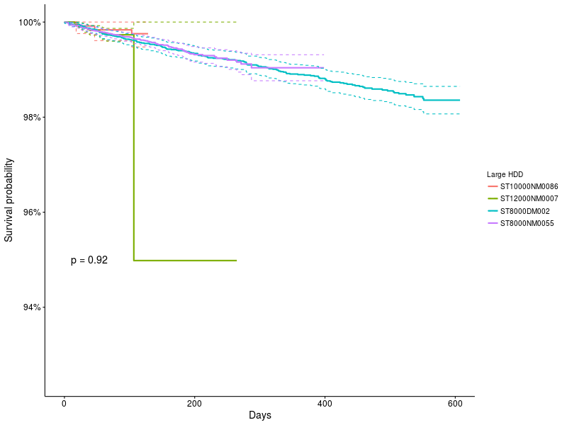
Chart 5 : Survival functions for large drives.

The KM method shows that there is no difference between them, despite the strange leap for the model ST12000NM0007

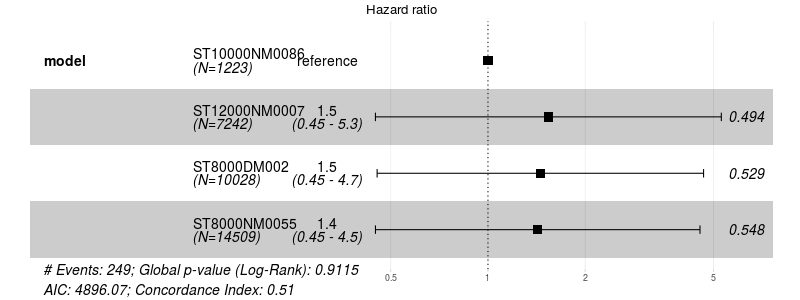
Chart 6 : Coke model for large drives, there is no statistical difference.

If we want to compare the ten most popular drives, we get the following picture:

Chart 7 : Survival Functions for the Top 10 Drives

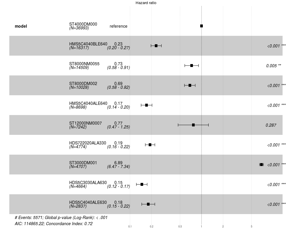
Chart 8 : Coke model for the 10 most popular drives

The most reliable: HDS5C3030ALA630, HMS5C4040ALE640, HDS5C4040ALE630, HDS722020ALA330, HMS5C4040BLE640, you can make a pairwise comparison (pairwise_survdiff function, if you are interested, is there a difference between them.

Parametric models

If it is interesting for us not just to compare different models of drives, but to answer a more specific question of the type: after what period of time one of the twenty disks in my file server will fail, then parametric models come to the rescue.

The simplest case is a model with constant risk; it assumes that throughout the life of the accumulator, the chance to die in a given period of time is approximately the same. For example, this model describes the process of decay of radioisotopes. In the literature, it is called the exponential model, because the survival function is described by the formula

$$

$$S (t) = 1-exp (-t * \ lambda)$$

When you calculate the% failure rate of drives for a year, then you use this model in an implicit way.

In practice, it is known that mechanical systems are better described by the Weibull function, with the formula

$$

$$S (t) = 1-exp (- (t * \ lambda) ^ p)$$

if p <1, then the probability of failures decreases with time, p = 1 - we have an exponential model and p> 1 - the probability of failures increases with time.

The survival package uses the survreg function to build this model:
For example, let's try building a Weibull model for 10 popular drives:

 fit_model_weibull<-survreg(Surv(age_days, status) ~ model, data=hdd_common) 

Compare with the exponential model

 fit_model_exp<-survreg(Surv(age_days, status) ~ model, data=hdd_common,dist='exponential') 

And let's see how the predicted distribution function coincides with the non-parametric KM, using the example of ST4000DM000 .

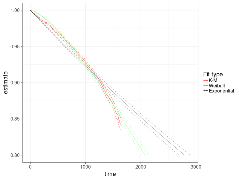
Chart 9 : Comparison of two parametric models with non-parametric models using the example of ST4000DM000

It can be seen that the Weibull model better describes the process of drive failure.
Models can be compared statistically using the Akaike information criterion:

  AIC(fit_model_weibull,fit_model_exp) df AIC fit_model_weibull 11 112208.8 fit_model_exp 10 112951.3 

A model with a lower AIC value — better describes the observed data.

And let's see the expected time of failure of 10% of drives:

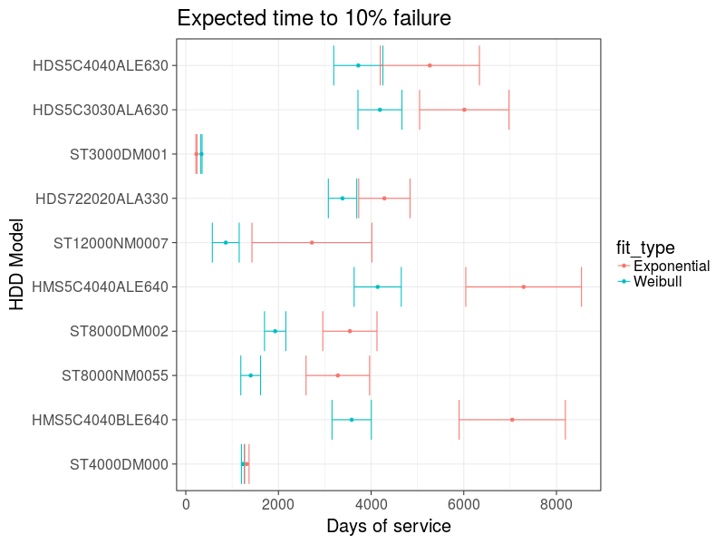
Chart 10 : Estimation of the failure time of the 10 most popular drives

On the assessment it is clear that the Weibul model gives an earlier estimate of the output of drives. By the way, if you simply calculate %% of the output of the drives out of operation every year, you get an approximation of an exponential model, which in this case gives an overestimated result.

Conclusion

So, with the help of freely laid out data on drive failures, you can predict future spending on disk replacement.

In the dataset from backblaze there is a lot of interesting information, for example, you can see how the temperature mode (parameter SMART 194) during drive operation affected its lifespan, or how the number of write cycles (parameter 241)

Scripts and .csv file for calculations is available on github .

If you are interested, you can download the sqlite database somewhere with the entire backblaze database (2.7GB after XZ packaging)

References

• Wikipedia: Survival analysis
• survminer: Survival Analysis and Visualization
• Michael J. Crawley. The R Book, 2nd edition ISBN: 978-0-470-97392-9