Hi, Habr! I present to your attention the translation of the article " Animal detection in the jungle - 1TB + of data, 90% + .

Or what we learned how to win prizes in such competitions, useful tips + some trivia

Tldr

The essence of the competition - for example, this is a random video with a leopard. All videos last 15 seconds, and there are 400 thousand ...

Final results at 3 am, when the competition ended - I was on the train, but my colleague submitted the application 10 minutes before the end of the competition

If you are interested to find out how we did it, what we learned, and how you can participate in such a one, then please under the cat.

0. Criteria for choosing the competition and the structure of the post

In our blog, we have already written how and why to participate in competitions.

Regarding the choice of this competition, it can be said that at the end of 2017 most of the competitions on the Kaggle were not so interesting and / or gave too little money at almost zero or so learning value and / or were with 100+ participants who sent their results on the first day because the last competitions were not so difficult. Just make 20 models on your own. The most vivid examples from the last one are interesting only in theory, and are nothing more than a casino with a GPU instead of chips.
For these reasons (a decent prize, the lack of strong marketing support due to 100+ simple applications on the first day, challenge, interestingness and novelty) - we chose this competition .

In a nutshell - you have ~ 200k videos for learning, ~ 80k videos for the test (and 120k untagged videos!). Videos are marked entirely, in 24 classes of animals. That is, video N has a certain class of animal (or its absence). That is, video1 is class1, video2 is class2, etc.

In this competition, I participated along with the subscriber of my telegram channel ( channel , webcast ). For brevity, this post will be structured as follows:

• TLDR section for people who want to quickly see working solutions and links;
• Code and jupyter laptops that are available here . The code is encapsulated and laptops use Jupyter extensions (codefolding, table of content, collapsiblle headers) for readability - but almost no attention was paid to turning the code into a tutorial, so read at your own risk;
• All the code I wrote was written in Pytorch, my colleague mainly used Keras.

1. TLDR1 - initial naive approach + collection of useful links on the topic

To get started, I put together a list of useful links in the order in which you probably should read them in order to solve a similar problem. To begin with, you should be familiar with computer vision, basic mathematics (linear algebra, mathematical analysis and numerical methods), machine learning and basic architectures in it.

2. TLDR2 - the best working approaches. Our pipelines and other prize winners

2.1 Best Practices

Our (3rd place):

Approximately half of the competition, I teamed up with Savva Kolbachev. Initially, before moving on to full-size videos, I tried some pieces with motion detection, gluing several 64x64-sized videos into one image, matrix decomposition. Sawa tried to use LSTM + some basic encoders for 64x64 video, as he had a car with a 780GTX card so he could only use micro data (64x64 3GB 2FPS), but even that seemed to be enough to score good points for hitting in the top 10 list.

Under the spoilers it will be possible to see briefly (in more detail below) our final pipeline and pipeline of the first place. And all sorts of other things.

What we missed / tested incorrectly, again more detailed below

When we trained the end-to-end model (pre-trained by Imagenet encoder + pre-trained GRU) - we got low error on the training set (0.03) and high on validation (0.13), which we considered a weakness of this approach. It turned out that Dmytro got the same results, but nevertheless finished the experiment. We abandoned this approach due to time constraints, but when we needed to make a selection of features from the pre-trained grid, I got more or less the same thing on my tests, but Sawa did not get the necessary values ​​on his pipeline. This led to the fact that we spent the last week trying to use new encoders instead of donating what we have already received. We also did not have time to try the additional training of encoders that we used. And try to train pooling / attention for the features that we got from the encoders.

An example of improvements that we tried - no increase compared with the conventional approach.

2.2 Key killer features, eureka and counter-intuitive moments

3. Basic data analysis and description, metrics

3.1 Dataset

Basic analysis can be found here . As I said before, the whole dataset weighs 1TB and the organizers of the competition shared it through a torrent, but you could download it directly (but rather slowly)

There were three versions of dataset available:

• Full 1TB
• Approximately 3GB of 64x64 video with 2FPS - surprisingly enough to achieve 75-80% accuracy and 0.03 points!
• 16x16 version.

In general, dataset was of good quality - each video was poorly annotated, but considering the size, it was still good - responsive support, it was possible to swing through torrents (although it was dammed quite late with one seeder in the USA), and the validation part was just the coolest thing I've seen. Our validation was always about 5% less than what we received on the board. The whole competition took 2 months, but in my case it took 2-3 weeks only to download and unpack the archive.

3.2 Basic analysis

To be honest, I didn't really understand much about dataset, simply because it was huge, but it was easy to get some key insights.

Some pictures of basic analysis

Actually dataset

Class labels - data is very unbalanced. On the other hand, train / test was made cool - so the distribution was the same here and there.

Some distributions

Main component analysis - easy to distinguish day and night

Video size in bytes on the log10 scale. Video without animals (blue) and with animals (orange). No wonder - due to compression, videos without animals are smaller

3.3 Metric

$$$$ display $$ AggLogLoss = - \ frac {1} {MN} \ sum_ {m = 1} ^ {M} \ sum_ {n = 1} ^ N [y_ {nm} \ log (\ hat y_ {nm} ) + (1-y_ {nm}) \ log (1- \ hat y_ {nm})] $$ display $$

Metric is just the average logloss for all 24 classes. This is good because there is such a metric in almost every DL package. It is quite easy to get normal points with her at once, but at the same time she is unintuitive and beloved. Very sensitive to the slightest amount of false positive predictions. Well, just adding new models improves this metric, which is not very good in theory.

4. How we solved the problem and our solution

4.1 Featureing

As we noted earlier, I selected features from different pre-trained models, like resnet152, inception-resnet, inception4 and nasnet. We found that it is best to select features not only from the last layer before fully connected, but also from skip-connections.

We also identified metadata like the width, height, and size of both datasets, micro and original. Interestingly, their combination works much better than just the original dataset. As a rule, metadata was very useful for identifying empty / non-empty videos, because empty videos usually weighed significantly less. This made it possible to separate more than 25% of empty videos, which, by the way, is the largest class in terms of number:

4.2 Division of training and validation samples

The distribution of classes was very unbalanced. For example, for the "lion" there were only two examples from the entire ~ 200k sample! Moreover, these were videos with several animal tags, so this needed to be done in a more specific split. Fortunately, we had the Planet code from the Planet: Understanding the Amazon from Space competition . With such a break, our test score was always a bit worse on the board than on the board:

def multilabel_stratified_kfold_sampling(Y, n_splits=10, random_state): train_folds = [[] for _ in range(n_splits)] valid_folds = [[] for _ in range(n_splits)] n_classes = Y.shape[1] inx = np.arange(Y.shape[0]) valid_size = 1.0 / n_splits for cl in range(0, n_classes): sss = StratifiedKFold(n_splits=n_splits, shuffle=True, random_state=random_state+cl) for fold, (train_index, test_index) in enumerate(sss.split(inx, Y[:,cl])): b_train_inx, b_valid_inx = inx[train_index], inx[test_index] # to ensure there is no repetetion within each split and between the splits train_folds[fold] = train_folds[fold] + list(set(list(b_train_inx)) - set(train_folds[fold]) - set(valid_folds[fold])) valid_folds[fold] = valid_folds[fold] + list(set(list(b_valid_inx)) - set(train_folds[fold]) - set(valid_folds[fold])) return np.array(train_folds), np.array(valid_folds) 

4.3. What we tried to do

After selecting the features, we had a matrix for each video of the form (45.3000), where 45 is the number of frames, and 3000 is the number of features for each frame.

What we tried and added to the final solution:

• We started with different RNNs, but they did not give us the best points and took a lot more time to learn (even for Keras, the implementation of CuDNN). But we used several trained RNNs in the final architecture.
• Using RNN, we decided to try attention and this gave us a good improvement. At first, we used this implementation on top of 2xCuDNNGRU with simple features. But as soon as we learned that the removal of the RNN does not greatly impair the results, we began to spend more time searching for different Keras implementations of attention and found this one . Attention worked for us like learnable pooling, which allowed us to move from matrix size (45,3000) to vector video size 3000.
• Max-min pooling gave a consistent increase in points and it worked much better than the default max \ avg pooling. The idea was to get a better idea of ​​how features change over time.
• Combining features from different models gave a better result, but it took more time and resources to learn.
• Training a separate model for recognizing empty / non-empty videos. This gave a slightly better result for this particular class, but it was meaningful, since the class was the most numerous.
• Pseudo-marking (splitting) has always given a bit of growth for our models. Usually the training went on a plateau after 12-15 epochs. It seems that the pseudo-markup introduced some variety to the training and improved validation.
• Stakanie models)

What we tried, but it did not work to solve the problem:

• Focal loss: in general, it works quite well and adds some variety to the models, but was not very useful according to the competition metric. But we will definitely try this for other projects.
• Deal with unbalanced classes: does not help according to metrics.
• 1D / 3D Convolutions
• Optical flow

4.4 Description of the final solution

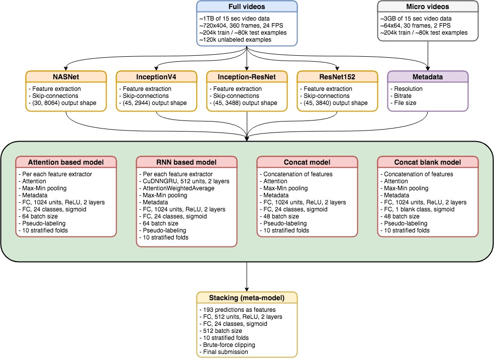
We trained 9 models, each with 5 folds, using dedicated features:

• 3 CuDNNGRU models with AttentionWeightedAverage and Max-Min polling layers based on resnet152, inception-resnet and inception4.
• 4 models with Attention and Max-Min pooling layers based on resnet152, inception-resnet, inception4 and nasnet.
• 1 concat model with Attention and Max-Min pooling layers (similar to the previous ones) but combined features from resnet152, inception-resnet, inception4.
• 1 concat model only for empty \ not empty predictions.

We found that 15 epochs + 5 epochs for pseudo-markup should be enough to get a pretty decent result. The batch size was 64 (44/20) for single-feature models and 48 (32/16) for nasnet and concat models. In general, the larger batch was better. Size selection depended on I / O disk and learning speed. For the final result, the predictions from the models were put together through 2 fully connected layers of the metamodel using 10 folds.)

We trained 9 models, each with 5 folds, using dedicated features:

• 3 CuDNNGRU models with AttentionWeightedAverage and Max-Min polling layers, based on resnet152 , inception-resnet and inception4 .
• 4 models with Attention and Max-Min pooling layers based on resnet152 , inception-resnet , inception4 and nasnet .
• 1 concat model with Attention and Max-Min pooling layers (similar to previous ones) but combined features from resnet152 , inception-resnet , inception4 .
• 1 concat model for empty / non-empty predictions only.

We found that 15 epochs + 5 epochs for pseudo-markup should be enough to get a pretty decent result. The batch size was 64 (44/20) for single-feature models and 48 (32/16) for nasnet and concat models. In general, a bigger batch was always better. Size selection depended on I / O disk and learning speed. To get the final result, the predictions from the models were put together through 2 fully connected layers of the metamodel using 10 folds.

5. Alternative approaches

As far as we know, a couple more things could have been done. For example, try detecting objects on 64x64 video, making bboxes and translating them to full-size videos. Make this two-three phased pipeline. Or try building bboxes from pre-trained models, but this is extremely difficult.

We did more or less detect the objects, but decided not to go this way, because we considered it unreliable - we didn’t want to waste time on manual marking because of the huge amount of data, plus we didn’t believe that even 64x64 motion detection would be stable.

6. Basic Tips for Competitors

• Try simple approaches
• Be sure you understand what works and why it works.
• Read all relevant paperwork on the topic, but do not spend too much time on one of the approaches if you are not sure that
  
  • it can be quickly and easily realized
  • you are sure that it will work
  • you can more or less combine the models from the works without implementing complex models from scratch
• Not afraid of the complexity of the problem. Modern libraries give you super power
• 90% of what is written in the paper is garbage. You do not have six months to test everything that you find. In these works, the form is usually valued rather than the practice.
• Combining models should be done only at the very end, and then as the last thing you can think of
• Communicate with people, cooperate. This is something like a stack of people) Together you study not twice as fast, but at ten.
• Share your code and approaches.

7. Basic Tips for Research and Production Models

• In 95% of cases, there are no stacks - usually it gives no more than 5-10%
• Your model and pipeline should be short, quick and convenient for engineers.
• All of the above is applicable for these purposes, but only taking into account the increased requirements for deployment.

8. Our equipment

We used 3 machines - my weak server with 1070Ti, but when we put the SSD there, it became limited by the size of the disk space. There was also a Savva car with a weak GPU and a server of my friends with two 1080Ti.