Richard Hamming: Chapter 14. Digital Filters - 1

“The goal of this course is to prepare you for your technical future.”

Hi, Habr. Remember the awesome article "You and your work" (+219, 2372 bookmarks, 375k readings)?



So Hamming (yes, yes, self-checking and self-correcting Hamming codes ) has a whole book based on his lectures. We translate it, because the man is talking.

')

This book is not just about IT, it is a book about the thinking style of incredibly cool people. “This is not just a charge of positive thinking; it describes the conditions that increase the chances of doing a great job. ”



We have already translated 16 (out of 30) chapters.

Chapter 14. Digital Filters - 1

(For the translation, thanks to Maxim Lavrinenko and Pakhomov Andrey, who responded to my call in the “previous chapter.”) Who wants to help with the translation - write in a personal or mail magisterludi2016@yandex.ru



Now that we have studied computers and figured out how they present information, let's turn to how computers process information. Of course, we will be able to study only some of the ways of their application, so we will focus on the basic principles.



Most of what computers process are signals from different sources, and we have already discussed why they are often in the form of a stream of numbers obtained from a sampling system. Linear processing, the only one for which I have enough time in the framework of this book, implies the presence of digital filters. To demonstrate how everything happens in real life, first I will tell you about how I began to work with them, and further about what I did.



First, I never went to the office of my vice president, V. O. Baker; we met only in the corridors, and usually stayed just a few minutes to talk. One day, around 1973-1974, when I met in the corridor, I told him that I remember that when I went to Bell Telephone Laboratories in 1946, the company gradually moved from relay to electronic central management, and many employees then they were transferred to other units, because they could not switch to oscillographs and other latest electronic technologies. For him, they represented only serious economic losses, but for me it was also a social loss, since these employees were at least unhappy that they were transferred (although this was their own mistake). I further mentioned that I observed a similar situation when we switched from old analog computers (for which there were many experts at Bell Telephone Laboratories, since they were developing most of the technologies during World War II) to more modern digital computers - we again a large number of engineers were lost, and again they were both an economic and social loss.



Then I noticed that we both know that the company is going to switch completely to digital signal transmission in the shortest possible time, with the result that we will get even more disgruntled engineers. Thus, I came to the conclusion that we must now do something to improve the situation, for example, to get elementary textbooks and other training materials in order to facilitate the adaptation of employees and lose fewer of them. He looked me straight in the eye and said, "Yes, Hamming, you must do this." And left! Moreover, he continued to encourage me through John Tukey, with whom he spoke often, so I knew that he was following my efforts.



What to do? At first, I thought I knew very little about digital filters, and, moreover, in fact, they did not interest me. But is it reasonable to ignore your vice president, as well as the persuasiveness of your own observations? Not! Possible social losses were too big for me not to attach importance to them.



Therefore, I turned to my friend Jim Kaiser, one of the world experts in the field of digital filters of that time, with a proposal to suspend his current research and write a book about electronic filters, arguing that summing up is a natural step in the development of any scientist. After some pressure, he agreed to write a book, and I thought that I was saved. But observing what he did showed that he did not write anything.



To save my plan, I made him the following suggestion: if he would teach me at breakfast in a restaurant (there would be more time to think than in the dining room) to help write a book together (at least the first part), then we will release it is by Kaiser and Hamming. He agreed!



After some time, I took a lot of knowledge from him, and the first part of the book was ready for me, but he still did not write anything. So one day I said: “If you don’t write anything, the authorship of the book will ultimately be listed as Hamming and Kaiser.” And he agreed. As a result, when I finished writing the book, but he never wrote anything, I said that I could thank him in the preface, but only Hamming would be listed as the author, he agreed - and despite this, we are still good friends ! So there was a book about digital filters, which I wrote, and which ultimately went through three editions, always with good advice from Kaiser.



Also, thanks to the book, I visited many interesting places, as I had spent short, weekly courses for many years. I started giving short courses as I wrote the book, as I needed feedback, and I suggested that the Expansion Department of the University of California at Los Angeles (UCLA) let me conduct training courses, and they agreed. This led to years of teaching at UCLA, once in Paris, England - London and Cambridge, as well as in many other places in the USA and at least twice in Canada. Doing what needed to be done, although I didn’t want to do it, ultimately paid off.



We now turn to the more important part - how I began to study a new subject - digital filters. Learning a new subject is something that you have to do many times in your career if you want to be a leader and not stay behind the latest developments. It soon became clear to me that in the theory of digital filters, Fourier Rows predominate, which I had just studied in college. In addition, I had a lot of additional knowledge due to my signal processing work done for John Tukey, who was a professor from Princeton, a genius, and one or two days a week by a Bell Telephone Laboratories employee. For almost ten years, most of the time I was his computing machine.



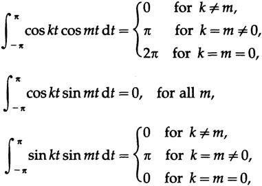
As a mathematician, I knew, like all of you, that any complete system of functions would be just as good for decomposing an arbitrary function into a series like any other complete system of functions. Why, then, are the Fourier series so different? I asked different electrical engineers, but I could not get satisfactory answers. One of the engineers said that the alternating currents were sinusoidal, so they used sinusoids, to which I replied that this made no sense to me. So much for the usual education of a typical electrical engineer after graduation!



Therefore, I should have thought about the basic principles, as I already did when using a computer with error detection. What actually happens? I believe many of you know that what we want is a time-invariant representation of signals, because there is usually no way to establish the beginning of a signal. Therefore, as a tool for representing things, we come to trigonometric functions (eigen transfer functions) in the form of both Fourier series and Fourier integrals.



Secondly, the linear systems that interest us at this stage have the same eigenfunctions — the complex exponents that are equivalent to real trigonometric functions. Therefore, a simple rule: if you have either a system with an invariant in time or a linear system, then you must use complex exponentials.



With further deepening of the topic, I found a third reason for using them in the field of digital filters. There is a theorem, which is often called the “Nyquist discretization theorem” (it was believed that it was known long before and was even published by Whittaker in a form that can hardly be understood even if you know the Nyquist theorem), which says that you have a signal with a frequency limited spectrum and you take samples at regular intervals with a frequency of at least twice the maximum frequency in the signal spectrum, then the original signal can be recovered from the received samples without loss. Consequently, the sampling process does not lose any information when we replace a continuous signal with equidistant reports, provided that the quantization levels cover the whole line of real numbers. The sampling rate is often referred to as the “Nyquist frequency” in honor of Harry Nyquist, also known for his contribution to the stability of servos, as well as other things. If you sample a function with an unlimited width of the spectrum, then the higher frequencies “overlap” with the lower ones. This term was introduced by Tukey to describe the phenomenon when one higher frequency appears later as a lower frequency in the Nyquist range.



The same is not true for any other set of functions, say degrees t. With a time-uniform sampling and subsequent signal recovery, one high degree of t will become a polynomial (consisting of several members) of lower degrees of t.

Thus, there are three good reasons for using Fourier functions: (1) invariance in time, (2) linearity, and (3) restoring the original function from its discrete representation is simple and straightforward.



Therefore, we will analyze signals in terms of Fourier functions, and I do not need to discuss with electrical engineers why we usually use complex exponents instead of real trigonometric functions to represent frequencies. We have a linear operation, and when we put a signal (a stream of numbers) into the filter, another stream of numbers is output. Naturally, if not from the course of linear algebra, then from other subjects, such as the course of differential equations, the question arises, what functions enter and leave without changes, except for the scale? As noted above, they are complex exhibitors; these are eigenfunctions of linear, time-invariant, discrete systems with time-uniform discretization.



And after all, how, the famous transfer function is the eigenvalues ​​of the corresponding eigenfunctions! When I asked various electrical engineers what the transfer function was, nobody told me about it! Yes, when they were told that this was the same thing, they had to agree, but they themselves, it seems, never thought about it! In their minds there was one and the same idea, but in two or more different images, and they did not even suspect any connection between them! Always start with the basic principles!



Now let's discuss “What is a signal?”. In nature, there are many signals that are continuous and which we sample at regular intervals and then digitize (quantize). Signals are usually a function of time, but any experiment in a laboratory that, for example, uses a voltage change with the same pitch and captures the corresponding responses, is also a digital signal. Thus, a digital signal is a sequence of measurements taken at regular intervals, represented as numbers. And we get at the output of the digital filter another set of numbers equidistant from each other. Processing and irregularly spaced data is allowed, but I will not consider them here.



Quantizing a signal to one of several output levels often has a surprisingly small effect. You have all seen images quantized into two, four, eight, or more levels, and even an image of two levels can usually be recognized. I will not consider quantization here, because it usually has a small effect, although at times it is very important.



The consequence of a uniform sampling time is the overlap, the frequency above the Nyquist frequency (which has two counts in the cycle) will be superimposed on the lower frequency. This is a simple consequence of the trigonometric identity.







where a is the positive remainder after removing an integer number of rotations, k (we always use rotations when discussing results and use radians in calculations, just as we use decimal and basic natural logarithms), and n is the number of steps. If a > 1/2, then we can write







Thus, the superimposed range will be less than 1/2 turn, plus or minus. If we use two real trigonometric functions, sin and cos, then we get a pair of eigenfunctions for each frequency, and the rotation range will be from 0 to 1/2 turns, and using complex exponential notation, we get one eigenfunction for each frequency, but Now the range will be from -1/2 to 1/2 turns. This avoidance of multiple eigenvalues ​​is one of the reasons why complex frequencies are much easier to process than real sine and cosine functions. The maximum sampling rate for which no overlap occurs is two counts per cycle, which is called the Nyquist frequency. The original signal cannot be recovered from counts in the superimposed frequency range, only frequencies that fall in the non-superimposed frequency interval (from -1/2 to ½) can be uniquely determined. The signals from the different superimposed frequencies go over to one frequency in the range and add algebraically; this is what we get as a result of the discretization. Thus, during an overlay, a certain frequency may be amplified or suppressed, and we cannot receive the original signal from the overlap signal. At the maximum sampling rate, the result for 1 cannot be said, as the non-superimposed frequencies must be within the range.



We will stretch (compress) the time so that we can measure the sampling rate as 1 count per unit of time, because it makes everything much easier and allows you to spread data from milli and microseconds to such intervals that can take several days or even years between readings. It is always wise to adopt the standard number system and the structure of thinking from one area to another - one application may allow finding a solution to a problem in another. I made sure that it makes a lot of sense to do this wherever possible - remove extraneous factors of scale and go to the original expressions. (But then I was originally studying math)



Overlaying is a fundamental discretization effect, and it has nothing to do with signal processing. It was convenient for me to think that as soon as samples are taken, all frequencies are in the Nyquist range, and therefore we do not need to draw periodic extensions of something, since other frequencies no longer exist in the signal - after sampling high frequencies go to the lower range and cease to exist. How wrong I was! The act of discretization produces a superimposed signal, with which we must work.



Now I come to three stories in which only ideas of discretization and overlay are used. In the first story, I tried to calculate a numerical solution of a system of 28 ordinary differential equations, and I had to know what sampling frequency I need to use (the decision step size is the sampling frequency that you use), because if it were half as large, than expected, the calculation counter will be approximately twice as large. In the most popular and practical methods of numerical solution, mathematical theory calculates the step size by the fifth derivative. Who could have known about this? No one. But if we consider a step as part of discretization, the overlap begins with two samples for the highest frequency, provided that you have data from minus to plus infinity. I intuitively understood that if there was only a short range of a maximum of five data points, I would need about twice as many, or 4 counts per cycle. And finally, with the availability of data on the one hand only, another doubling factor is possible; only 8 counts per cycle.



Then I did two things: (1) developed a theory and (2) conducted numerical tests on a simple differential equation







Both of them showed that with 7 counts per cycle, you get an approximate accuracy (per step), and with 10 counts it is absolute. So I explained everything as it was and requested higher frequencies in the expected solution. The validity of my request was assessed, and after a few days I was told that I should worry about frequencies up to 10 cycles per second, and those above are not my concern. And it was right, and the answers were satisfactory. The discretization theorem in action!



The second story touches a story told to me by chance in the halls of Bell Telephone Laboratories, that some West Coast subcontractor had problems with simulating the launch of the Nike rocket, he used intervals between 1/1000 and 1/10 000 seconds. I immediately laughed and said that this must be some kind of mistake, because for the model they used, it would be enough from 70 to 100 samples. It turned out that they had a binary number shifted 7 positions to the left, 128 times more! Debugging a large program at the other end of the continent using the discretization theorem!



The third story is about how a group in a naval graduate school lowered the frequency of a very high-frequency signal so as to be able to sample it, according to the discretization theorem, as they understood it. But I realized that if they intelligently sampled a high frequency, then sampling itself would lower the frequency of the signal (impose the original signal on the lower part of the spectrum). After several days of disputes, they still removed the rack with the equipment to lower the frequency, and then the rest of the equipment began to work better! And this time, I only needed a firm understanding of the overlay effect upon discretization. This is another example of why you need to know the basic principles well; you can easily think out the rest and do things that no one has ever told you.







Figure 14.I



Discretization is a fundamental approach that we use when processing data in the process of working with digital computers. Now that we understand what a signal is and what sampling does with a signal, we can safely move on to a more detailed examination of signal processing.



We first discuss non-recursive filters whose purpose is to pass through some frequencies and suppress others. For the first time, a similar problem arose in the telephone company when they had the idea that if you move all the frequencies of one voice message to the top (modulate a signal), beyond the frequency range of another voice message, then these two signals can be folded and sent together using the same wires, and on the other side they can be filtered and divided, and then move the frequencies of the higher signal to the usual frequency range (demodulate). This frequency shift is simply multiplication by a sinusoidal function and the choice of one of two frequencies (single-band modulation), which arise according to the following trigonometric identity (this time we use real functions)





() , .



, , , u(t)=u(n)=u _n , — y _n





C _j =C _-j ( C ₀ ).



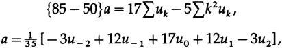
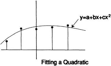
I need to remind you about the least squares method, because it plays a fundamental role in what we are going to do, for this I will develop a smoothing filter to show you how filters are created. Suppose that we have a signal with the addition of "noise" and it needs to be smoothed out, to remove the noise. I believe that it will seem reasonable for you to approximate 5 consecutive values ​​of a straight line by the least squares method, and then take the average value on this line as the “smoothed function value” at this point.



For mathematical convenience, we will select 5 points at t = -2, -1,0,1,2 and draw a

straight line, fig. 14.I.







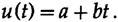
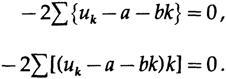
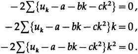
The least squares method says that we must minimize the sum of the squares of the differences between the data and the points on the line, i.e. minimize







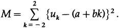
What parameters need to be used to differentiate to find the minimum? These are a and b, not t (now a discrete variable k) and u. The line depends on the parameters a and b, and this is often

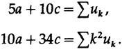
a stumbling block for students; equation parameters are variables to minimize! Therefore, when differentiating with a and b and equating the derivatives to zero to get the minimum, we have







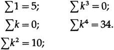
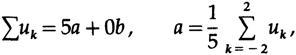
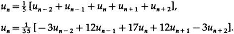
In this case, we need only a - the line value at the midpoint, therefore, we use (some sums are indicated for later use),







from the upper equation we have







. , a, , . 14.II, 1/5, ; , , «» – . .



2k+1 , , .



, , . 14.III:







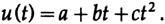
a, b c, :







a. ( a)







c, , 17 -5 ,







« » , , . , , , , .





14.II







14.III



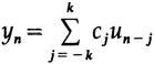
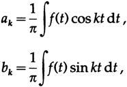
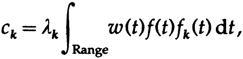
n, :











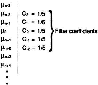
Now let's ask ourselves what will be at the output if we put a pure own function at the input. We know that since the equations are linear, they must return their own function, but multiplied by the eigenvalue corresponding to the frequency of the eigenfunction - the value of the transfer function at that frequency. Taking the upper part of the two formulas, we





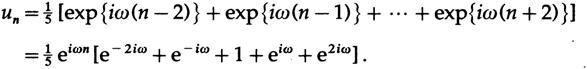
apply the elementary trigonometry and obtain the eigenvalue at the frequency ω (transfer function):







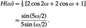
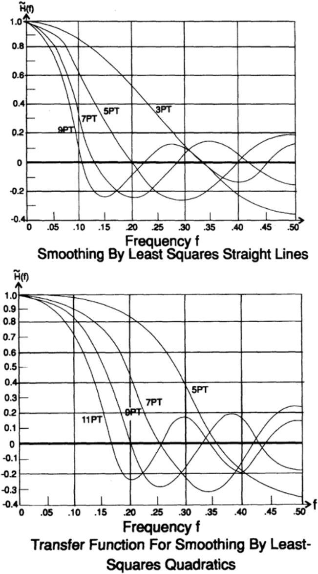
In the case of parabolic smoothing we get:







These transfer characteristics for smoothing 2k + 1 values ​​are easy to sketch, fig. 14.IV.



Smoothing formulas have a central symmetry in their coefficients, and the differentiating formulas have an odd symmetry. From the obvious formula







, , . , .



, ( ) , — . , .



. , f (t)





( ):











a ₀ /2 , a _k k= 0. , , .



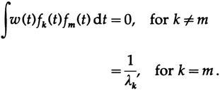
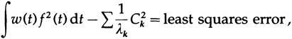
, . {fk(t)} w (t)≥0.











14.IV



,







Where





, - .



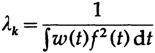
C _k ( C) . We have







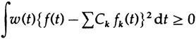
. C _m





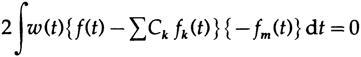
, Ck=ck. , .



,





, . , . , .



To be continued...



Who wants to help with the translation - write in a personal or mail magisterludi2016@yandex.ru



By the way, we also launched another translation of the coolest book - “The Dream Machine: The History of Computer Revolution” )