The motive for this publication was the report “Using the R Software for Log File Analysis” at the USENIX conference, which was discovered on the Internet when searching for answers to the next questions. Since the whole printed article was written, it is logical to assume that the topic is relevant. Therefore, I decided to share examples of solving such problems, the solution of which was not given such importance. In fact, “margin notes”.
R is, indeed, very well suited for such tasks.

It is a continuation of previous publications .

Analytics for Squid

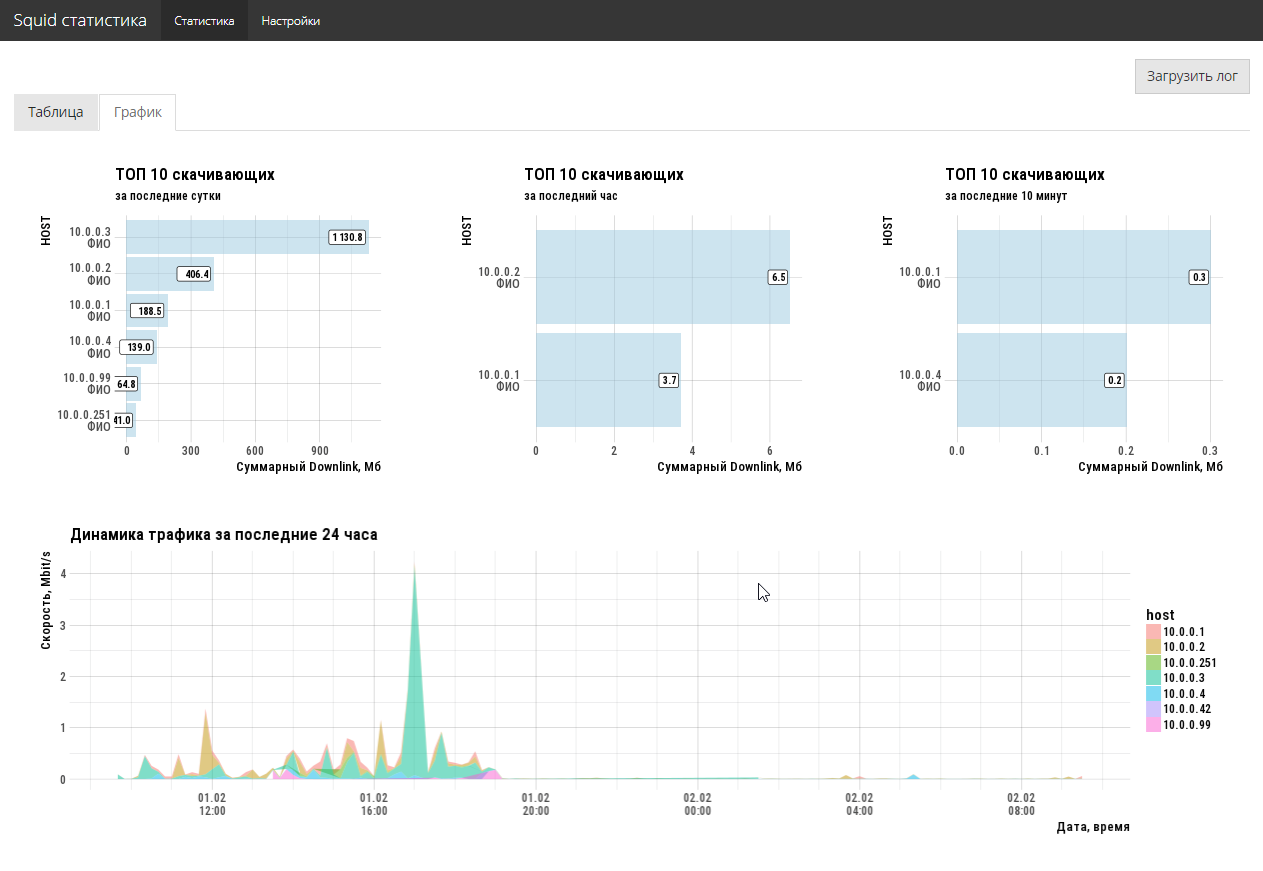
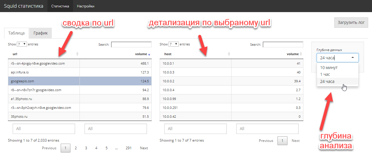
Task setting is quite simple. The network administrator needs to quickly know who and how much downlink traffic is consumed, which sites are the main absorbers and who goes there. A big story is not needed, you need a cut, maximum, for the last week. Experiments with various open-source analyzers did not bring joy to the administrator (everything is missing).

OK. We provide free access via http to the access.log file (squid), take R and make an interactive shiny application. Unfortunately, the special webreadr package on CRAN did not work, but it does not matter. tidyverse + hands solve an import task in 5 lines. For convenience, we publish the resulting application on a shiny free server.

3-4 hours of work and the problem is solved. Moreover, with a full-fledged graphical UI, and not just a hardcore command line. 2 screen codes completely solve the task of the administrator.

Application code here . Naturally, the code is not optimal, but no such task was set, it was necessary to quickly close the immediate problem.

Custom System X Analytics

The problem would not be worth attention if a few points:

• System X consists of several components that write several different types of log files;
• data scattered across several tens of thousands of files;
• the type of the log file is somewhat far from the normalized view and it is very difficult to eat it in a direct stream.

A fragment of the contents of one of these files (the number of nodes in general form may vary over time):

 2017-12-29 15:00:00;param_1;param_2;param_2;param_4;param_5;param_6;param_7;param_param_8;param_9;param_10;param_11;param_12 Node 1;20645;328;20308;651213;6258;644876;1926;714;1505;541713;75;541697 Node 2;1965;0;1967;89820;236;89605;419;242;396;27714;44;27620 2017-12-29 15:05:00;param_1;param_2;param_2;param_4;param_5;param_6;param_7;param_param_8;param_9;param_10;param_11;param_12 Node 1;20334;1039;19327;590983;2895;588234;1916;3673;1507;498059;347;497720 Node 2;1701;0;1701;89685;259;89417;490;424;419;26013;93;25967 

Probably, the author of such a format of the log file was guided by high motives, but now it is extremely problematic to analyze such creativity on a computer with standard tools.

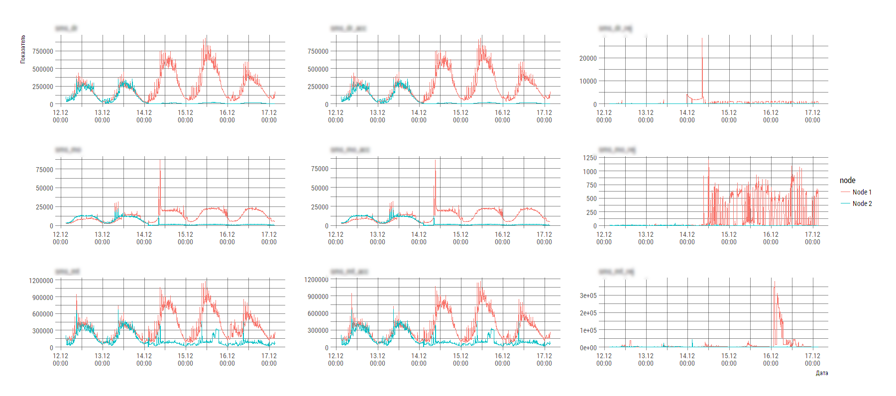
But it is not scary when there are R. in the hands. To understand the motives and write a cunning parser on regulars is lazy and there is no time, we use the data science scrap. tidyverse all with raw materials and we use tidyverse tools for cutting / transformation. All business on two screens of code and a couple of hours of work (analyze, think, download, draw graphics, draw conclusions).

 loadMainData <- function(){ flist <- dir(path="./data/", pattern="stats_component1_.*[.]csv", full.names=TRUE) raw_df <- flist %>% purrr::map_dfr(read_delim, col_names=FALSE, col_types=stri_flatten(rep("c", 13)), delim=";", .id=NULL) df0 <- raw_df %>% #         mutate(tms=ifelse(X2=="param_1", X1, NA)) %>% fill(tms, .direction="down") #       data_names <- df0 %>% slice(1) %>% unlist(., use.names=FALSE) df1 <- df0 %>% # ,       , # ,   ,      purrr::set_names(c("node", data_names[2:13], "tms")) %>% mutate(idx=row_number() %% 3) %>% filter(idx!=1) df2 <- df1 %>% mutate(timestamp=anytime(tms, tz="Europe/Moscow", asUTC=FALSE)) %>% mutate_at(vars(-node, -timestamp), as.numeric) %>% select(-tms, -idx) %>% select(timestamp, node, everything()) main_df <- df2 %>% tidyr::gather(key="key", value="value", -timestamp, -node) main_df } 

At the output we get such a picture (imbalance of the system is clearly visible), according to which the engineer is already specifically beginning to deal with System X.

PS Technique has now gone such that you can neglect the optimization of the execution time at the stage of primary development. To work with log files with a cumulative volume of several gig, a laptop with 8 GB RAM is enough and it takes about one or two minutes to process, analyze and draw.

Previous publication - “HR-analytics” by means of R.