We count chickens until they are pecked
This story began with a short article in the New York Times about Luke Robitail, a 13-year-old high school student from Euless, Texas, who won the Raytheon Mathcounts National Competition, correctly answering the following question:
The next day, Jordan Ellenberg tweeted such a task:
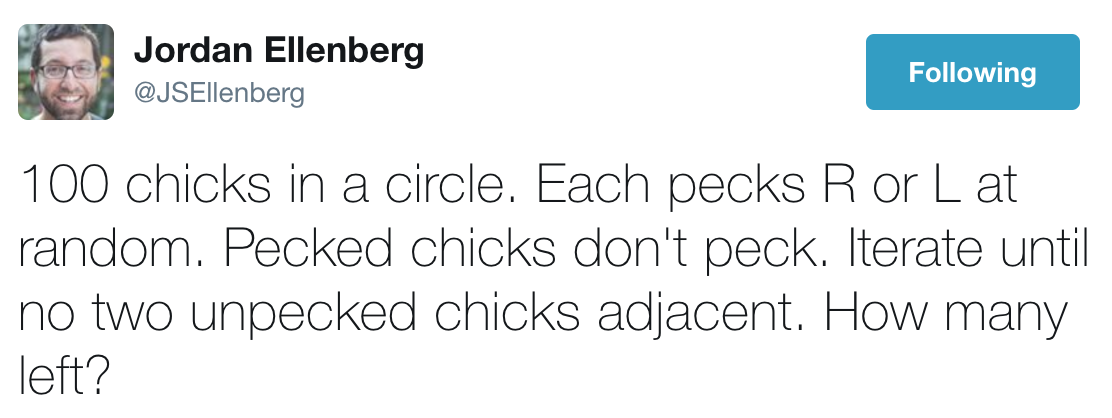
“100 chickens are sitting in a circle. Each pecks randomly R or L. Pecked hens do not bite anyone. Iterations are carried out until two adjacent, unhewed chickens remain. How many chickens are left? ”
')
I do not need to fit this story in 140 characters, so I will supplement the question of Ellenberg with details in the way I understood it. The original task was related to a single iteration of synchronized random pecking, and now we have several iterations. During one iteration, each chicken randomly turns left or right and bites one of its neighbors. However, if the chicken has already been pecked, it will never bite again, even it continues to peck. If two neighboring hens peck at each other in the same iteration, both of them fly out of the game for all subsequent rounds. If a non-banned chicken turns out to be between two pecked, it will never be pecked, and therefore it can peck endlessly. The question is, how many chickens will survive and become “invulnerable”?
Below are the spoilers, so now you can try to answer the question yourself. While you are doing this, I will talk a little about chickens and about the rhetoric and semiotics of mathematical "word problems".
My only knowledge of poultry is taken from a trip to my aunt Norette’s farm in southern New Jersey. I can not say that my experience is great, but it is worth noting that I have never seen hens sitting around, pecking at each other in a random way. (They have a pecking order !) Moreover, I never noticed something in their social interactions that resembled the “turn the other cheek” principle that chickens from the described task demonstrate. Why does a pecked chicken never bite again? This is an even bigger mystery than a quantitative question that we have to answer. Has the chicken suddenly discovered wisdom and the power of non-resistance to violence? I have another explanation, but it is not suitable for sensitive people: perhaps pecked hens do not bite back because pecks kill outright.
I know that it’s foolish to demand a real story from a similar story. Mathematical word problems belong to a genre in which nobody expects likelihood. They occur in a world where liars always lie, and knights always tell the truth, where shipwrecked sailors are obsessed with the possibility of divisibility of a mountain of coconuts, where people do not know the color of the hat they are wearing. Even the laws of physics lean toward mathematical needs: a fly flying between two converging trains instantly changes its direction. These chickens sitting in a circle are not fluffy clumps of yellow fluff; they are mathematical abstractions. They have no feathers, but they have coordinates and state variables.
I am quite satisfied with the abstraction; let's get rid of redundant details by any means. However, isn’t the meaning of word problems the idea of associating mathematics with some aspects of the experience familiar to readers? Recall the ancient famous problem of crossing a river, in which a wolf cannot be left with a goat, which in turn cannot be left with cabbage (approx.: In the original, a fox, a chicken and a bag of corn). These restrictions are easy to understand if you know something about the taste preferences of wolves and chickens. However, such intuitive help is not applicable to the pecking problem. On the contrary, the more we know about the true behavior of birds, the more confusing this task will be.
Anyway. Let's get started! Do you already have your own answer?
The one-iteration task from the Mathcounts Competition competition comes down to the oldest trick in the probability theory textbook. The hen remains unclipped only if both its neighbors have turned away and pecked in the other direction. The probability of avoiding pecking left and right is f r a c 1 2 . These two events are independent; therefore, the probability of remaining undetected on both sides is equal to f r a c 1 2 t i m e s f r a c 1 2 = f r a c 1 4 . This reasoning applies equally to all the birds in the circle, so one should expect that 25 percent of the chickens will remain intact.
Do you agree with this analysis? When I read an article in the Times , I got to it pretty quickly (of course, not at all so quickly to get ahead of Luke Robitail, who pressed the button). But then I started having doubts. Is it strictly true that the neighbors of the chicken on the left and on the right are completely independent? In the end, they are linked by a chain of other chickens. It is possible that some influence may spread around the circle, creating correlations between the left and right hens and changing the probability of survival.
It is time to experiment: write the program and run the simulation. We will line up a ring of 100 unbilled chickens and perform one iteration of random simultaneous pecking. Repeat many times and calculate the average number of non-spat birds. (Here is a brief entry: let N - the number of chickens in the ring, and S - the number of remaining uncircumcised. I will designate as b a r S average value S averaged after R repetitions of the experiment.) My results:
As expected, the mean is pretty close to the 25 survivors. Moreover, each time the sample size increases by 100 times, the approximation accuracy increases by about ten times. This pattern corresponds to the empirical rule of statistics: fluctuations of a random process are proportional to the square root of the sample size. That is a slight deviation from b a r S = 25 look like an innocent random noise, and not some sort of systematic bias.
That is the question solved, is not it?
In general, the simulation looks pretty convincing for a particular case. N = $ 10 chickens, but the result may differ for other N values. In particular, it is possible that there is a certain effect of finite dimensionality that becomes apparent only for small N. Consider the "circle" of only two chickens. In this simulation, the left and right neighbor is the same chicken! Regardless of the randomly made choices, the two hens immediately peck at each other, and some of the survivors will be equal not to 25 percent, but to zero.
The next, larger “circle” consists of three chickens collected in a triangle. Two neighbors now are different chickens, but they are also neighbors of each other. What happens when three chickens pounce on each other? The system has 2 3 = 8 possible combinations of pecking, and we can easily learn from everything. The arrows on the diagram show which side of the chicken they chose to peck at.

In two cases, all the hens peck to the left or peck to the right, and there are no survivors. In every other case, exactly one chicken is left behind. By collecting all eight combinations, we get six out of 24 hen-hens, that is, the ratio is b a r S = f r a c 1 4 . That is, it seems that the anomaly of the final values affects only the case of a problem with two chickens.
But wait! There is another possible factor distorting the results. Can we be sure that the same results will be for even and odd numbers of chickens? For any odd N value, there is only one way to kill all the chickens in one round: they must all peck in the same direction. However, with even N , another combination leads to immediate extinction: neighboring chickens are divided into pairs and pecked each other. Will this additional method change the overall survival probability?
Let's see what happens when N = 4. Now there is 2 4 = 16 possible outcomes:

As expected, there are no survivors in the four combinations. On the other hand, there are also four combinations in which not one, but two non-stick hens remains. Additional losses and additional winnings balance each other in a miraculous way. In total, we will have 16 survivors of 64 chickens, that is, the ratio is again equal to b a r S = f r a c 1 4 .
After this long and winding walk around the combinatorics of chick pecking, we returned exactly to where we started. The likelihood of not being whipped up after one iteration of pecking is frac14 for anyone N gt2 . All my worries about finite size effects and even-odd unevenness were a waste of time. So why did I share them with you? Although my worries turned out to be unreasonable, they were not at all contrived. Even small changes in the order of pecking will lead to different results. For example, pecking will be consistent, not simultaneous. One selected chicken starts a sequence of pecks, and then other birds, located clockwise from it, make their moves. When the chicken's turn comes, then if it has already been pecked, then it does nothing. If it is not pecked, she pecks left or right, choosing randomly. The iteration ends when each chicken makes its move.
With N=2 it is easy to see that the first pecking chicken always survives, and the other always dies, that is, the survival rate is equal to frac12 . By counting the hens on paper a little, you can see that the 50 percent survival rate is also valid for N=3 . In the study of large values N computer experiments show that the survival rate N to infinity again approaching frac12 . However, between these limit values, there are funny situations:

With N=4 the proportion of survivors falls below 0.47. (The exact probability is frac3064=0.46875 .) This is the minimum of values. But when the ratio returns to 0.5, oscillations appear in the curve, showing discrepancies in the results for even and odd quantities: the probability of survival decreases more for even N than for odd N. This was the behavior I was looking for (but did not find) in the original version of the problem from the Mathcounts competition.
Let's again take on the Ellenberg problem of iterative pecking (with simultaneous, not sequential pecking). We already know that after the first iteration, we can expect that about a quarter of the chickens will remain unfulfilled. Obviously, the part of the unqualified cannot increase after several iterations. That is, in the final state, the expected proportion of survivors barS must be somewhere between zero and frac14 .
It will be useful to look at the usual configuration of pecked (●) and non-pecked (○) chickens after one iteration of synchronized pecking:
(Mentally connect the left and right ends of the array to create a ring.) Notice that there are long lines of sticking chickens, but non-strayed chickens are present in only two configurations. They are either singles (● ○ ●) or pairs (● ○○ ●). The reason for this pattern is simple to understand. After a round of pecking, the existence of a group of three non-spit hens in a row (● ○○ ●) is impossible. The average hen is obliged to peck left or right, that is, she cannot have two unclipped neighbors.
Such restrictions simplify the analysis of subsequent iterations. Singles are essentially immortal and immutable: the never-thrown chicken in the middle will never bite again, and the never-beaten neighbors will never be returned to the “non-stick” state. For couples, there are four possible scenarios, corresponding to the four ways that two active hens choose to peck:

In any iteration, all these four events have the same probability, namely frac14 . The first three resulting states are final , in the sense that further iterations of pecking will not change them. In the fourth case, we again have a pair of neighbors, before which in the next iteration the same choice of options will appear. Over time, when the number of iterations will tend to infinity, the fourth case should lead to one of the other results, and therefore in the long run we should consider the probability of the fourth case to be zero, and the probability of each of the other three cases to be frac13 .
Now it is time to put these contingent events together and calculate the probability of a chicken’s survival in the long run. The figure below shows the diagram. In the first round of pecking, three-quarters of the chickens are immediately destroyed. Of the remaining quarter, half are loners who survive endlessly. Every other surviving hen is a member of the pair, and the other pecking hen from her pair is her left or right neighbor.

In the lower part of the scheme, the effect of all successive iterations is summarized, which continues until all pairs are destroyed or reduced to single ones. (I call it pecking to the last .) For each path leading to the survival of a loner, the probability is the product of the individual probabilities encountered along the way. There are three such paths with probabilities. frac18 , frac148 and frac148 and amount frac16 .
I must confess that I failed to carry out this analysis - or to get the right answer - on the first attempt. I achieved it only after running the simulation, thus learning what I need to look for. And even then I had problems with double counting.
Here are the results of the simulation:
Note that accuracy is again improved as the square root of the sample size, despite the fact that the variance here is greater than in the experiment with one iteration.
What about finite size effects? In a circle with only two or three chickens, their fate is completely determined by a single iteration of pecking: barS respectively 0 and frac14 . That is, these smallest circles do not comply with the rule frac16 but it seems that circles of any larger size come down to frac16 . There are no differences even odd in them.
Another approach to understanding the problem of iterated chick pecking is Markov chain theory. For the ring of N chickens we list everything 2n states and assign the probability of each transition between states. Consider a ring of four chickens, which has 16 states. Symmetry allows us to combine some of the states; other states can be discarded because they are unattainable from the initial state with four non-pecked hens ( ).
).
In the model, only four states marked with a red outline should remain. Transitions between them are written in a directed graph, in which each arrow is labeled with an appropriate probability. It is worth noting that the initial state there are only outgoing arrows; after leaving it is impossible to return there. States  and
and  are absorbing : the only outgoing arrow leads back to the same state; that is, once in one of these states, you will not get out of it.

Important information from this directed graph can be displayed in the matrix 4 times4 , in which the rows and columns are marked with four states, and the elements of the matrix represent the probability of transition from the row state to the column state. The sum of the elements of each row is 1, as it should be if they are probabilities.

The pattern of zero elements in the transition matrix implies that some states cannot be reached from other states, even indirectly. For this reason, it is said that the Markov model is irregular . This is a bit annoying, because regular Markov models are easier to analyze and understand. In a regular model, when we take successive powers of the transition matrix, it reduces to a steady state in which all rows are the same, and each column consists of a single recurring value. This fixed state represents the distribution of probabilities in the long run. An irregular Markov model may not even have an established limiting distribution, but it does exist in ours, and this gives us certain clues. Any ring of four chickens should result in one of two absorbing states. With a two-thirds probability, this final state will be and with probability one third . This result corresponds to the calculated one-sixth lobe of unbilled chickens.
That is, you can sum up, right? Both in the problem from the competition, and in its iterative version of Ellenberg, the expected number of surviving chickens was asked, and we answered: N chickens expected number of survivors barS equally fracN4 after a single iteration of pecking and fracN6 when pecking to the end. However, ironically, the expected value of the probabilistic process does not necessarily tell us what to expect. Consider a simple task: tossing a coin 100 times, how many “eagles” do we expect to see? The obvious answer is 50, and it is true in the sense that no other number is more able to correctly predict the result of an experiment. However, the probability of seeing exactly 50 “eagles” is only 0.08, that is, in 90 percent of cases we will receive another number.
Instead of looking only at the expected value, let's examine the range of possible values S games with pecking. We have already established that zero survivors is a possible result, that is, we have a lower limit. What about the upper limit - the maximum number of survivors? In the process with one iteration of pecks, each chicken makes, that is, after this iteration, each chicken must have at least one pecked neighbor. Based on this fact, I declare that a surviving population can never be greater fracN2 . (Do you agree? It took me some time to convince myself of this.)
If a S can never be more fracN2 , then the next question will be: can it ever reach this limit? And if we can have the same number of salted (●) and non-strayed (○) chickens, how will they be located in the ring? It seems logical to suggest the following configuration:
This is a stable state: unheralded chickens can never bite, that is, no further changes are possible. And the survival rate is frac12 . But this scheme has a problem: it cannot be reached from the initial state. Look at any of the pecked chickens and ask the question: which of the neighbors pecked her? Obviously, neither of them, because no one had pecked them both. But this is impossible, because each chicken in the first iteration should peck.
Although we excluded the scheme from alternate black and white chickens, we are on the right track. There is another configuration in which, after the first iteration, half of the chickens also remain, and this scheme is reachable from the initial state:
When we connect the ends to get a ring, each chicken, regardless of whether it was pecked or not, has one pecked neighbor. It turns out that this is the only way, apart from the obvious symmetric cases, in order to achieve 50 percent survival. (Strictly speaking, 50 percent can only be achieved when N divided by 4 but S never less fracN−22 .)
When pecking is done to a winning finish, the upper bound S= fracN2 no more reachable. Let's say we would try to keep fracN2 after a few iterations of pecking. Obviously, in the first iteration we would have to start with the maximum number of survivors
Does this mean that S= fracN4 is the highest possible value after pecking to the bitter end? No, it does not mean. There is another scheme in which one out of every three chickens survives:
This configuration is achievable in one iteration and is infinitely stable, because none of the pecking chickens has pecking neighbors. No other scheme has a greater density of survivors in the process of pecking to the end.
To summarize: after one iteration of pecking, the number of surviving chickens should be somewhere between zero and fracN2 and expected quantity barS - exactly in the middle, in fracN4 . After the completion of all subsequent iterations, the number of unheeded chickens will be in the interval between zero and fracN3 and the expected value will again be in the middle, barS= fracN6 .
“How many chickens will survive?” - this question seems to require a numerical answer, but in fact the most informative answer to it will be not a number at all, but a distribution :

Each curve captures the results of a million experiments with a ring of 100 chickens, showing the frequency of each possible value. S . As expected, the distribution at one iteration has a peak at 25 survivors, and the task curve with iteration at 17 (the closest to frac1006 whole). Notice that the red curve is not only shifted to the left, but also higher and narrower.
To better see the results, let's change the scale. To make the curves smoother, I will move to experiments with N=$10,00 chickens The green curve is for one iteration, and the red one is for an experiment with many iterations of pecking:


With larger values N curve peaks are at 2500 and 1666.67, that is, exactly at the points expected for fracN4 and fracN6 . It was not surprising to find peaks at these points, but what controls the width and overall shape of the curve? In other words, what is the mathematical nature of the distributions?
The first guess is always to try a normal (or Gaussian) distribution. For the pecking task, the normal distribution determines P(s) the probability of observation S survivors, as follows:
A rather convoluted equation for such a familiar concept, but one can single out the main meaning from it. The equation defines a symmetric curve with a peak, where S equally mu , that is, the mean value of the distribution. Peak width depends on standard deviation sigma . Since the area under the curve is constant, sigma essentially determines its height: a narrower peak should be higher.
We can reconcile the normal distribution with the pecking data using a procedure that finds the optimal values. mu and sigma , such that minimize the discrepancy between the data points and the mathematical model. In the two graphs below, the agreed models are superimposed on two data graphs, the first for one iteration, the second for iterations to the end:


The agreement looks quite close, the theoretical curves separate the experimental ones from beginning to end. In a sense, this result can be considered a success, but I still do not find such an approach to the problem completely satisfactory. The normal curve creates a very good descriptive model of the pecking process, but does not predict or explain it. Do not forget that we agreed the curve with the data, and not vice versa. I do not see obvious ways to create some normal distribution from what I know about the interactions of pecking chickens. In particular, where do the values come from sigma two models? Why sigma approx25 in a model with one iteration but sigma approx23.6 in a model with many iterations? These values look like independent parameters that we have to adjust to fit the data. Moreover, they will be different for each value. N . Another problem: a normal curve is a continuous distribution defined on the whole real number axis. The pecking function is discrete; it makes sense only for integer values.
Let's lay aside the normal curve and consider another plausible model: the binomial distribution, which is discrete and occurs in many contexts related to probabilities. Suppose we throw 10,000 bones and count how many of them have a unit. When we repeat the experiment many times, the expected number of units will be one sixth of 10,000, that is, the same value as the expected number of survivors in an iterative experiment with pecking chickens. For bones, there is a well-known mathematical expression that defines not only the expected value, but also the shape of the entire distribution. Suppose that each bone has a probability of ejection 1 indicated by p . We will throw N bones and we need to know the chance to see k units = for any k from 0 before N . The formula for processing this information is:
Here pk(1−p)N−k gives the probability of any single combination k units among N bones. Binomial coefficient N choosek equal to N!/k!(N−k)! \), calculates the number of such combinations.
With N=$10,00 and p= frac16 we get a curve showing the result of the above mentioned bone-throwing experiment. Perhaps the same curve describes what happens in the pecking model with many iterations, which has the same expected value? Alas, but no.

The binomial curve is wider and flatter than the distribution of survivors of iterated pecking. What went wrong? When I first saw the chart, I had a hunch. As stated above, the binomial coefficient N choosek counts all the choices k items from a variety of size N . It is suitable for experimenting with bones, because all possible combinations k success among N equally likely. In particular, when we throw 10,000 bones, we may not see any units at all or see all 10,000 bones with units on the top face; the entire result interval has a probability greater than zero.
The task with pecking is different, 100 percent of chickens can’t stay ned. That is, only a subset is achievable. N choosek combinations. If the binomial distribution will work in such a context, we need to somehow change it to include only achievable results.
Thinking that it is easier to solve the problem, if you already know the answer, I tried to play around with the distribution parameters to see how the schedule would react. I tried to fit the curve into a narrower and higher graph, keeping centering on the same mean value. Average equals Np , that is, if we reduce N then we will have to increase p by the same ratio. Here are the results of some experiments:

The dark green curve is the one we have already seen for the binomial distribution with N=$10,00 and p= frac16 . Change parameters on N=5000 and p= frac13 seems like a step in the right direction, but N=3333 and p= frac12 turn out to be even better. Then try N=$250 and p= frac23 ldots Bingo! The yellow curve perfectly matches the pecking data. That is, it seems we can predict survival in the ring of pecking from N members by creating a binomial distribution with parameters N prime= fracN4 and p prime=4p .
I can repeat the same trick to find the binomial distribution corresponding to one iteration of pecking. This time the magic numbers bending the curve along the desired trajectory are equal N′= fracN3=$333 and p′=3p= frac34 .

In contrast to the normal distribution, the binomial model is constructive (that is, it is able to predict). Of two parameters N′ and p′ we can calculate both the mean of the distribution and the standard deviation. Mean is just N′p′ standard deviation is sqrtN′p′(1−p′) . For example, when 10,000 chickens average mu turns out to be equal 1666.666 dots (as expected) and the standard deviation sigma equally 23.570226 . (Have a fitted normal distribution sigma=23.567337 .) For the case of one iteration mu equally 2500 , but sigma equally 25 . (To avoid rounding errors, I took N equal to 9999 , but not 10,000 .)
Well, hooray? At least, we have a formula for calculating the shape and location of the distribution of chick pecking, which depends only on a pair of parameters; N′ and p′ . But I grumble again, in fact, I'm even more angry. Maybe the model explains the data, but how to explain the model itself? With 10,000 chickens and survival probabilities in the first iteration frac14 why the formula is needed N′=$333 and p′= frac34 ? Where do these numbers come from? And why in the case of multiple iterations are suitable N′=2500 and p ′ = 23 ?
It is inconvenient for me to say how much time I spent on hopeless blundering in the swamps of probability theory, trying to solve these riddles. (I even turned to the recently published book The Probability Lifesaver (“Lifeguard in the world of probabilities”) , which I highly recommend, but it did not save me.) In search of answers, I investigated polynomial binomial generalizations. I studied the convolutions of distributions and calculated conditional probabilities. I filled the whole notebooks with straight lines from ● and ○ in search of patterns that could explain such mysterious fractionsN3 paired with3four and N4 paired with23 .Every night I went to bed with a promising idea, but then I woke up and found a significant drawback in it.
Now it seems to me that I have the right explanation. It came to me after many checks over several evenings. I will talk about it, but only at the very end of the article. You might be able to find it earlier. In the meantime, I want to expand the horizons of the task about chickens.
Our cozy circle of chickens is a one-dimensional structure. In the ring you can go clockwise and against it, there are no other significant directions in this small universe. Now imagine that instead of planting all the chickens in a circle, we put them in a grid, that is, in an array of rows and columns, filling in the area of two-dimensional space. In order not to leave the last chickens along the edges of the square array, we can connect the left edge with the right one, and the top one with the bottom one. (In terms of topology, this turns a rectangle into a torus.) Making real chickens in this experiment work together would be even more difficult than in the one-dimensional version, but we do not care; we have long said goodbye to our barn reality.
The most important thing in this two-dimensional arrangement is that each chicken now has not two, but four neighbors. There are more hostile neighbors, so one would expect the chicken to be more vulnerable to attacks. On the other hand, each of these neighbors distributes its pecks to potential victims, whose number has doubled. How are these competition conditions balanced?
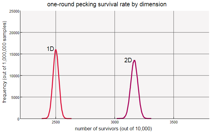
With a single iteration of pecking, we can calculate the probability of survival just as in a one-dimensional system. A hen remains unclarified only if all its neighbors peck in some other direction. Each neighbor bites so with probability34 , so the probability that they all turn away is equal to( 34 )4 .Numerically, this turns out to be about 0.3164, (in a circle, the value was 0.25). That is, the proportion of surviving in two dimensions is more than one; distraction to a greater number of victims outweighs the danger of a greater number of attackers. The distribution observed in computer experiments confirms this result.
Here it is shown how the chicken net 40 × 40 looks after one iteration of pecking.

In a two-dimensional array is 1600 chickens. If we count the unchallenged, we find that there are 501 of them, that is, the number of survivors is 0.3131, and this is close to the theoretical value of 0.3164. Simulations confirm that the expected survival rate is equal to( 34 )4for gridsN × N for any valueN more2 . (For mesh 2 × 2 the proportion of survivors is equal toone4 , as in the one-dimensional system. And there is a reason for this!)When I looked intently at the scheme presented above, I noticed a certain repeating texture with chains of ○ dividing the spots ●. This may be an illusion, but I do not think so. In two dimensions, the restriction "no three in a row" is removed; the array contains rows and columns with up to six consecutive non-jerked hens, as well as diagonal lines. But a solid block
3 × 3 of non-henched chickens () we will not see here, and even crosshairs 3 × 3 (
  ).Such patterns cannot exist, because a hen in the middle of a block must peck at one of its four neighbors. In a more general sense, the system is still limited by the rule: each hen, pecked or unkept, must have at least one pecked neighbor.
Since the first iteration of pecking in a two-dimensional world survives more chickens, it seems plausible that with the continuation of iterations to completion a large proportion of chickens can survive. Let's try an experiment:

In this array 40 × 40 turned out to be 238 surviving from 1600 chickens, which islessthan the proportion of survivors in one dimension (one sixth). With a sample of one million such grids, I found that the average proportion of survivorsˉ S is approximately equal to 0.1533. Compare the distribution in one-and two-dimensional systems:

When moving from 1D to 2D, the peak shifts to the left, and the average moves from 0.1667 to 0.1533. The two-dimensional hill is also slightly higher and narrower, that is, it exhibits less variance.
But why stop at two dimensions? Let's ask our chickens to gather in a three-dimensional lattice, and reconnect the opposite boundaries, creating a three-dimensional analogue of a toroidal surface. It is easy to guess what this experiment will lead to. In one dimension, each chicken had only two neighbors, and the percentage of survivors after one iteration of pecking was( 12 )2=1four . In two dimensions with four neighbors, the corresponding value was ( 34 )4=81256 . In a three-dimensional array, each chicken has six neighbors, that is, it is obvious to extrapolate as ( 56 )6=1562546656 , receiving the value≈ 0.3349 . After the simulation, these data are confirmed and demonstrate a clear trend when creating arrays of chickens with an increasing number of measurements.

Based on this series of results, we can safely summarize: when a chicken has n neighbors, the expected share of survivors after the first iteration of pecking is
By increasing n this expression converges to a value approximately equal to0.36787944 .Do we know this number? Sameonee . (By changing the minus to the plus, we get e , 2.71828 .) When I came to this formula, the sudden appearanceonee caught me off guard, although it shouldn't have. The constant appears in the same way as in the rumor propagation modelI wrote about afew years ago. What about an iterative pecking process with large quantities of measurements? With increasing measurements, the share of survivors steadily decreases:

The proportion of chickens, which have never been pecked, falls from 16.7 percent in one dimension, approximately two times, when we shove our chickens into a seven-dimensional space. In other words, a space with larger dimensions increases the initial share of survivors (after one iteration of pecking), but reduces survival in the long run (after pecking to the bitter end). Another way to demonstrate the effects of measurements is to track the average number of survivors after each iteration of pecking in spaces from one to seven measurements.

I can offer a rough rationalization of this trend. If you are a chicken in a one-dimensional ring, then your chance of survival after the first iteration of pecking is equal to the wholeone4 , but if you survive this iteration, then the chance to avoid pecking in the second iteration is no lessone2 .Why has it increased? Thanks to your own actions: your strike with a beak in the first iteration eliminated the threat from one of two neighbors. In subsequent iterations, the chances continue to grow: the longer you survive, the more likely you are to survive after the neighbors rest in peace.
The same trend persists in a larger number of measurements, but the magnitude of the effect decreases. For example, in four dimensions you have eight neighbors, and your chance of survival after the first iteration is equal to( 78 )8, or about 0.34. As you peck at one of these neighbors, the probability of surviving after the second iteration is higher, but not by much:( 78 )7, or 0.39.Looking at the graphs above, we can assume that as the number of measurements tends
D to infinity, the number of survivors (after pecking) will drop to zero. To explore this idea, we really do not need infinite dimensional space. The more important is not the geometric arrangement of chickens, but the number of neighbors, and we can approximate an infinite-dimensional grid, simply stating that all chickens are the closest neighbors. In other words, the “who bites whom” line becomesfull, in which arcs connect each hen to all others. It seems like a recipe for total annihilation; you cannot be safe as long as at least one chicken continues to peck. But the details of the end of the game give little room for variations. Will there be one survivor, or they will not be at all?Peter Winkler considered a similar task - “Group Russian Roulette” in the book
Mathematical Puzzles: A Connoisseur's Collection (p. 33). The elements of this version of the game are not chickens, but “armed and angry people” participating in simultaneous shooting rounds at random neighbors. Winkler concludes that the probability of survival does not approach the limit with increasingN .I do not see this effect in a problem with chickens: there is always only one surviving hen. It seems to me that the difference lies in the fact that in Winkler’s roulette, players do not spend ammunition on enemies already shot, while chickens continue to peck at neighbors who are no longer responding.
Finally, I will return to the narrow bounds of one dimension and to the mysterious binomial distributions, which seem to predict the statistics of chick pecking in this system. I’ll repeat it briefly: if we throw 10,000 bones and count the ones that have fallen units, we expect to find approximately 1667. If we place 10,000 chickens in a circle and wait until they finish pecking, we expect approximately 1667 non-stray survivors. An experiment with bones is described by a binomial distribution with parametersN = 10,000 and p = 16 .The same model does not work for chickens: the predicted distribution is much wider than the observed one. But the oddity is not that. The real secret is why another binomial model with parametersN ′ = 2500 and p ′ = 23 seems to fit the experimental results. The fact that the model with the bones does not work in chickens does not surprise us. The most important assumption underlying the binomial distribution is that the events or objects counted are independent of each other. For bones, this is true; one single bone doesn't care what happens to the others. But in the circle of pecking hens the most important thing is interaction with neighbors. If you are pecked, then it changes the chances that your neighbors will ever be pecked. Independence enters the binomial distribution through a coefficient
( Nk ) . With N bones onk of which the unit fell out, all possible variants together with the unit are equally probable for all other bones; The binomial coefficient counts the number of such combinations. But atN chickens, of whichk is not pecked, the equiprobability of all combinations is not true. In fact, many schemes, for example, ○○○, are impossible. If interactions with neighbors spoil the binomial model when
N = 10,000 and p = 16 , how do these interactions win in models withN ′ = 2500 and p ′ = 23 ?The longest I was misled by the observation that 2500 is the expected number of survivors after one iteration of pecking, and that two thirds of these survivors are expected to survive in all subsequent iterations. Of course, the appearance of these two numbers in the binomial distribution cannot be a meaningless coincidence. Maybe not, but I managed to understand the situation only when I completely abandoned this line of reasoning.
We need a model in which we consider a combination of 2500 objects, where two thirds of the objects can be considered successful or surviving. I found such a model. Objects are not separate chickens, but groups of four chickens. Consider this set of four tuples:
If you randomly select elements from this set and connect them as a string, any sequence created will be the output of an iterated pecking process. A typical result is as follows:
Notice that this sequence satisfies all the rules for our heap of chickens, which are pecked to the bitter end. All uncleaned are loners, surrounded by nested neighbors. Each pair of ○ shares at least two ●, and this ensures that each element of the sequence has at least one neighbor ●. There is no way to concatenate any sample of elements a, b, and c that violate these rules. Moreover, if a, b and c are selected with equal probability, then the expected proportion of ○ in the sequence is equal to one6 .
I have deeply conflicting feelings for this discovery. On the one hand, it is always a joy to get to the very bottom of the problem that tormented you. On the other hand, we have here a simple recipe for creating a sequence with the same structure and statistics as the result of the pecking process, but it does not give us any hints about the nature of this process. There is no connection with the behavior of chickens. What is worse, it is not even a true and accurate model. Although it turns out that the curve coincides with the data, it is just an approximation. Proving it is very easy. Binomial distribution withN ′ = 2500 and p ′ = 23 has a maximum threshold in2500 . Any number of survivors more 2500 model gives zero probability, despite the fact that in the pack of10,000 can actually survive up3333 chickens This flaw becomes noticeable on a smaller model, for example, on such
N = 24 :

The predicted and observed curves show discrepancies everywhere, but take a close look at the right end of the distribution, where the binomial curve (violet) reduces to zero all survivors of more than six, while experimental data (red) include 6718 cases with seven survivors and 49 cases with eight survivors.
A similar model for a process with one iteration of pecking uses a multitude of four three-element tuples: It again generates a sequence that is very similar to the result of the pecking experiment, but it fails to reproduce the right side of the distribution. In the model, the maximum possible density of survivors is
one3 , while it should be equalone2 .
Perhaps you think that a funny task for high school students about pecking chickens is not worth an article for 8000 words with arguments about Markov chains and probability distributions, with tables, equations and 25 graphs and diagrams. It also occurred to me. However, I want to argue and say that these studies were not completely frivolous.
Mathematics is not obliged to give us beautiful, finite and single-line solutions to any problem, but we would deceive ourselves if we had surrendered too early. In the example from this article, computer simulations turned out to be simple and productive. By running the program for five minutes, I can get answers to many detailed questions, and I will not have serious doubts about the correctness of these answers. But they do not help me find the connection between microscopic mechanisms (random pecks of chicken left or right) and macroscopic observations (the distribution hasμ = 16 bσ = 23.56 ).Richard Hamming’s hackneyed quotation says that the purpose of the calculations is insight, not numbers, but I did not achieve insight.
Secondly, in fact, the problem is not about chickens, real or abstract. This is the door to many other multiparticle problems in statistical physics, dynamical systems, and cellular automata.
And finally, I was wondering, so what's wrong with that? Perhaps the fun will not end there. What about zombie chickens whose pecks bring other chickens back to life?
Postscript: Carl Whitti calculated the correct probability for the case with one iteration, let's give him the floor.
In the barn circle sit 100 chickens. Each of the hens randomly pecks its nearest neighbor to the left or to the right. What is the expected number of chickens that no one bites?Judging by the Times article, Robitail took less than a second to respond.
The next day, Jordan Ellenberg tweeted such a task:
“100 chickens are sitting in a circle. Each pecks randomly R or L. Pecked hens do not bite anyone. Iterations are carried out until two adjacent, unhewed chickens remain. How many chickens are left? ”
')
I do not need to fit this story in 140 characters, so I will supplement the question of Ellenberg with details in the way I understood it. The original task was related to a single iteration of synchronized random pecking, and now we have several iterations. During one iteration, each chicken randomly turns left or right and bites one of its neighbors. However, if the chicken has already been pecked, it will never bite again, even it continues to peck. If two neighboring hens peck at each other in the same iteration, both of them fly out of the game for all subsequent rounds. If a non-banned chicken turns out to be between two pecked, it will never be pecked, and therefore it can peck endlessly. The question is, how many chickens will survive and become “invulnerable”?
Below are the spoilers, so now you can try to answer the question yourself. While you are doing this, I will talk a little about chickens and about the rhetoric and semiotics of mathematical "word problems".
My only knowledge of poultry is taken from a trip to my aunt Norette’s farm in southern New Jersey. I can not say that my experience is great, but it is worth noting that I have never seen hens sitting around, pecking at each other in a random way. (They have a pecking order !) Moreover, I never noticed something in their social interactions that resembled the “turn the other cheek” principle that chickens from the described task demonstrate. Why does a pecked chicken never bite again? This is an even bigger mystery than a quantitative question that we have to answer. Has the chicken suddenly discovered wisdom and the power of non-resistance to violence? I have another explanation, but it is not suitable for sensitive people: perhaps pecked hens do not bite back because pecks kill outright.
I know that it’s foolish to demand a real story from a similar story. Mathematical word problems belong to a genre in which nobody expects likelihood. They occur in a world where liars always lie, and knights always tell the truth, where shipwrecked sailors are obsessed with the possibility of divisibility of a mountain of coconuts, where people do not know the color of the hat they are wearing. Even the laws of physics lean toward mathematical needs: a fly flying between two converging trains instantly changes its direction. These chickens sitting in a circle are not fluffy clumps of yellow fluff; they are mathematical abstractions. They have no feathers, but they have coordinates and state variables.
I am quite satisfied with the abstraction; let's get rid of redundant details by any means. However, isn’t the meaning of word problems the idea of associating mathematics with some aspects of the experience familiar to readers? Recall the ancient famous problem of crossing a river, in which a wolf cannot be left with a goat, which in turn cannot be left with cabbage (approx.: In the original, a fox, a chicken and a bag of corn). These restrictions are easy to understand if you know something about the taste preferences of wolves and chickens. However, such intuitive help is not applicable to the pecking problem. On the contrary, the more we know about the true behavior of birds, the more confusing this task will be.
Anyway. Let's get started! Do you already have your own answer?
The one-iteration task from the Mathcounts Competition competition comes down to the oldest trick in the probability theory textbook. The hen remains unclipped only if both its neighbors have turned away and pecked in the other direction. The probability of avoiding pecking left and right is f r a c 1 2 . These two events are independent; therefore, the probability of remaining undetected on both sides is equal to f r a c 1 2 t i m e s f r a c 1 2 = f r a c 1 4 . This reasoning applies equally to all the birds in the circle, so one should expect that 25 percent of the chickens will remain intact.
Do you agree with this analysis? When I read an article in the Times , I got to it pretty quickly (of course, not at all so quickly to get ahead of Luke Robitail, who pressed the button). But then I started having doubts. Is it strictly true that the neighbors of the chicken on the left and on the right are completely independent? In the end, they are linked by a chain of other chickens. It is possible that some influence may spread around the circle, creating correlations between the left and right hens and changing the probability of survival.
It is time to experiment: write the program and run the simulation. We will line up a ring of 100 unbilled chickens and perform one iteration of random simultaneous pecking. Repeat many times and calculate the average number of non-spat birds. (Here is a brief entry: let N - the number of chickens in the ring, and S - the number of remaining uncircumcised. I will designate as b a r S average value S averaged after R repetitions of the experiment.) My results:
| R | b a r S |
|---|---|
| 100 | 24.79 |
| 10,000 | 24,9881 |
| 1,000,000 | 25,000274 |
| 100,000,000 | 24,99991518 |
As expected, the mean is pretty close to the 25 survivors. Moreover, each time the sample size increases by 100 times, the approximation accuracy increases by about ten times. This pattern corresponds to the empirical rule of statistics: fluctuations of a random process are proportional to the square root of the sample size. That is a slight deviation from b a r S = 25 look like an innocent random noise, and not some sort of systematic bias.
That is the question solved, is not it?
In general, the simulation looks pretty convincing for a particular case. N = $ 10 chickens, but the result may differ for other N values. In particular, it is possible that there is a certain effect of finite dimensionality that becomes apparent only for small N. Consider the "circle" of only two chickens. In this simulation, the left and right neighbor is the same chicken! Regardless of the randomly made choices, the two hens immediately peck at each other, and some of the survivors will be equal not to 25 percent, but to zero.
The next, larger “circle” consists of three chickens collected in a triangle. Two neighbors now are different chickens, but they are also neighbors of each other. What happens when three chickens pounce on each other? The system has 2 3 = 8 possible combinations of pecking, and we can easily learn from everything. The arrows on the diagram show which side of the chicken they chose to peck at.
In two cases, all the hens peck to the left or peck to the right, and there are no survivors. In every other case, exactly one chicken is left behind. By collecting all eight combinations, we get six out of 24 hen-hens, that is, the ratio is b a r S = f r a c 1 4 . That is, it seems that the anomaly of the final values affects only the case of a problem with two chickens.
But wait! There is another possible factor distorting the results. Can we be sure that the same results will be for even and odd numbers of chickens? For any odd N value, there is only one way to kill all the chickens in one round: they must all peck in the same direction. However, with even N , another combination leads to immediate extinction: neighboring chickens are divided into pairs and pecked each other. Will this additional method change the overall survival probability?
Let's see what happens when N = 4. Now there is 2 4 = 16 possible outcomes:
As expected, there are no survivors in the four combinations. On the other hand, there are also four combinations in which not one, but two non-stick hens remains. Additional losses and additional winnings balance each other in a miraculous way. In total, we will have 16 survivors of 64 chickens, that is, the ratio is again equal to b a r S = f r a c 1 4 .
After this long and winding walk around the combinatorics of chick pecking, we returned exactly to where we started. The likelihood of not being whipped up after one iteration of pecking is frac14 for anyone N gt2 . All my worries about finite size effects and even-odd unevenness were a waste of time. So why did I share them with you? Although my worries turned out to be unreasonable, they were not at all contrived. Even small changes in the order of pecking will lead to different results. For example, pecking will be consistent, not simultaneous. One selected chicken starts a sequence of pecks, and then other birds, located clockwise from it, make their moves. When the chicken's turn comes, then if it has already been pecked, then it does nothing. If it is not pecked, she pecks left or right, choosing randomly. The iteration ends when each chicken makes its move.
With N=2 it is easy to see that the first pecking chicken always survives, and the other always dies, that is, the survival rate is equal to frac12 . By counting the hens on paper a little, you can see that the 50 percent survival rate is also valid for N=3 . In the study of large values N computer experiments show that the survival rate N to infinity again approaching frac12 . However, between these limit values, there are funny situations:
With N=4 the proportion of survivors falls below 0.47. (The exact probability is frac3064=0.46875 .) This is the minimum of values. But when the ratio returns to 0.5, oscillations appear in the curve, showing discrepancies in the results for even and odd quantities: the probability of survival decreases more for even N than for odd N. This was the behavior I was looking for (but did not find) in the original version of the problem from the Mathcounts competition.
Let's again take on the Ellenberg problem of iterative pecking (with simultaneous, not sequential pecking). We already know that after the first iteration, we can expect that about a quarter of the chickens will remain unfulfilled. Obviously, the part of the unqualified cannot increase after several iterations. That is, in the final state, the expected proportion of survivors barS must be somewhere between zero and frac14 .
It will be useful to look at the usual configuration of pecked (●) and non-pecked (○) chickens after one iteration of synchronized pecking:
●○●●●○○●●●●○●●○●●○○●●●○○●●●●●○●●●●●●●●●○○●●●●●●○○●●●○●●●●●●○●●●○○●●●●●(Mentally connect the left and right ends of the array to create a ring.) Notice that there are long lines of sticking chickens, but non-strayed chickens are present in only two configurations. They are either singles (● ○ ●) or pairs (● ○○ ●). The reason for this pattern is simple to understand. After a round of pecking, the existence of a group of three non-spit hens in a row (● ○○ ●) is impossible. The average hen is obliged to peck left or right, that is, she cannot have two unclipped neighbors.
Such restrictions simplify the analysis of subsequent iterations. Singles are essentially immortal and immutable: the never-thrown chicken in the middle will never bite again, and the never-beaten neighbors will never be returned to the “non-stick” state. For couples, there are four possible scenarios, corresponding to the four ways that two active hens choose to peck:
In any iteration, all these four events have the same probability, namely frac14 . The first three resulting states are final , in the sense that further iterations of pecking will not change them. In the fourth case, we again have a pair of neighbors, before which in the next iteration the same choice of options will appear. Over time, when the number of iterations will tend to infinity, the fourth case should lead to one of the other results, and therefore in the long run we should consider the probability of the fourth case to be zero, and the probability of each of the other three cases to be frac13 .
Now it is time to put these contingent events together and calculate the probability of a chicken’s survival in the long run. The figure below shows the diagram. In the first round of pecking, three-quarters of the chickens are immediately destroyed. Of the remaining quarter, half are loners who survive endlessly. Every other surviving hen is a member of the pair, and the other pecking hen from her pair is her left or right neighbor.
In the lower part of the scheme, the effect of all successive iterations is summarized, which continues until all pairs are destroyed or reduced to single ones. (I call it pecking to the last .) For each path leading to the survival of a loner, the probability is the product of the individual probabilities encountered along the way. There are three such paths with probabilities. frac18 , frac148 and frac148 and amount frac16 .
I must confess that I failed to carry out this analysis - or to get the right answer - on the first attempt. I achieved it only after running the simulation, thus learning what I need to look for. And even then I had problems with double counting.
Here are the results of the simulation:
| R | barS |
|---|---|
| 100 | 16,53 |
| 10,000 | 16.6835 |
| 1,000,000 | 16.664404 |
| 100,000,000 | 16.66701664 |
Note that accuracy is again improved as the square root of the sample size, despite the fact that the variance here is greater than in the experiment with one iteration.
What about finite size effects? In a circle with only two or three chickens, their fate is completely determined by a single iteration of pecking: barS respectively 0 and frac14 . That is, these smallest circles do not comply with the rule frac16 but it seems that circles of any larger size come down to frac16 . There are no differences even odd in them.
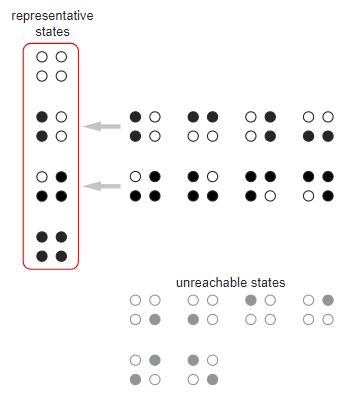
Another approach to understanding the problem of iterated chick pecking is Markov chain theory. For the ring of N chickens we list everything 2n states and assign the probability of each transition between states. Consider a ring of four chickens, which has 16 states. Symmetry allows us to combine some of the states; other states can be discarded because they are unattainable from the initial state with four non-pecked hens (
In the model, only four states marked with a red outline should remain. Transitions between them are written in a directed graph, in which each arrow is labeled with an appropriate probability. It is worth noting that the initial state
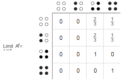
Important information from this directed graph can be displayed in the matrix 4 times4 , in which the rows and columns are marked with four states, and the elements of the matrix represent the probability of transition from the row state to the column state. The sum of the elements of each row is 1, as it should be if they are probabilities.
The pattern of zero elements in the transition matrix implies that some states cannot be reached from other states, even indirectly. For this reason, it is said that the Markov model is irregular . This is a bit annoying, because regular Markov models are easier to analyze and understand. In a regular model, when we take successive powers of the transition matrix, it reduces to a steady state in which all rows are the same, and each column consists of a single recurring value. This fixed state represents the distribution of probabilities in the long run. An irregular Markov model may not even have an established limiting distribution, but it does exist in ours, and this gives us certain clues. Any ring of four chickens should result in one of two absorbing states. With a two-thirds probability, this final state will be
That is, you can sum up, right? Both in the problem from the competition, and in its iterative version of Ellenberg, the expected number of surviving chickens was asked, and we answered: N chickens expected number of survivors barS equally fracN4 after a single iteration of pecking and fracN6 when pecking to the end. However, ironically, the expected value of the probabilistic process does not necessarily tell us what to expect. Consider a simple task: tossing a coin 100 times, how many “eagles” do we expect to see? The obvious answer is 50, and it is true in the sense that no other number is more able to correctly predict the result of an experiment. However, the probability of seeing exactly 50 “eagles” is only 0.08, that is, in 90 percent of cases we will receive another number.
Instead of looking only at the expected value, let's examine the range of possible values S games with pecking. We have already established that zero survivors is a possible result, that is, we have a lower limit. What about the upper limit - the maximum number of survivors? In the process with one iteration of pecks, each chicken makes, that is, after this iteration, each chicken must have at least one pecked neighbor. Based on this fact, I declare that a surviving population can never be greater fracN2 . (Do you agree? It took me some time to convince myself of this.)
If a S can never be more fracN2 , then the next question will be: can it ever reach this limit? And if we can have the same number of salted (●) and non-strayed (○) chickens, how will they be located in the ring? It seems logical to suggest the following configuration:
●○●○●○●○●○●○This is a stable state: unheralded chickens can never bite, that is, no further changes are possible. And the survival rate is frac12 . But this scheme has a problem: it cannot be reached from the initial state. Look at any of the pecked chickens and ask the question: which of the neighbors pecked her? Obviously, neither of them, because no one had pecked them both. But this is impossible, because each chicken in the first iteration should peck.
Although we excluded the scheme from alternate black and white chickens, we are on the right track. There is another configuration in which, after the first iteration, half of the chickens also remain, and this scheme is reachable from the initial state:
●●○○●●○○●●○○When we connect the ends to get a ring, each chicken, regardless of whether it was pecked or not, has one pecked neighbor. It turns out that this is the only way, apart from the obvious symmetric cases, in order to achieve 50 percent survival. (Strictly speaking, 50 percent can only be achieved when N divided by 4 but S never less fracN−22 .)
When pecking is done to a winning finish, the upper bound S= fracN2 no more reachable. Let's say we would try to keep fracN2 after a few iterations of pecking. Obviously, in the first iteration we would have to start with the maximum number of survivors
●●○○●●○○●●○○ . However, at least half of the unheeded chickens in this configuration should die in subsequent iterations, leaving no more fracN4 survivors.Does this mean that S= fracN4 is the highest possible value after pecking to the bitter end? No, it does not mean. There is another scheme in which one out of every three chickens survives:
●●○●●○●●○●●○This configuration is achievable in one iteration and is infinitely stable, because none of the pecking chickens has pecking neighbors. No other scheme has a greater density of survivors in the process of pecking to the end.
To summarize: after one iteration of pecking, the number of surviving chickens should be somewhere between zero and fracN2 and expected quantity barS - exactly in the middle, in fracN4 . After the completion of all subsequent iterations, the number of unheeded chickens will be in the interval between zero and fracN3 and the expected value will again be in the middle, barS= fracN6 .
“How many chickens will survive?” - this question seems to require a numerical answer, but in fact the most informative answer to it will be not a number at all, but a distribution :
Each curve captures the results of a million experiments with a ring of 100 chickens, showing the frequency of each possible value. S . As expected, the distribution at one iteration has a peak at 25 survivors, and the task curve with iteration at 17 (the closest to frac1006 whole). Notice that the red curve is not only shifted to the left, but also higher and narrower.
To better see the results, let's change the scale. To make the curves smoother, I will move to experiments with N=$10,00 chickens The green curve is for one iteration, and the red one is for an experiment with many iterations of pecking:
With larger values N curve peaks are at 2500 and 1666.67, that is, exactly at the points expected for fracN4 and fracN6 . It was not surprising to find peaks at these points, but what controls the width and overall shape of the curve? In other words, what is the mathematical nature of the distributions?
The first guess is always to try a normal (or Gaussian) distribution. For the pecking task, the normal distribution determines P(s) the probability of observation S survivors, as follows:
P(S)= frac1 sigma sqrt2 pi exp− frac12 left( fracS− mu sigma right)2
A rather convoluted equation for such a familiar concept, but one can single out the main meaning from it. The equation defines a symmetric curve with a peak, where S equally mu , that is, the mean value of the distribution. Peak width depends on standard deviation sigma . Since the area under the curve is constant, sigma essentially determines its height: a narrower peak should be higher.
We can reconcile the normal distribution with the pecking data using a procedure that finds the optimal values. mu and sigma , such that minimize the discrepancy between the data points and the mathematical model. In the two graphs below, the agreed models are superimposed on two data graphs, the first for one iteration, the second for iterations to the end:
The agreement looks quite close, the theoretical curves separate the experimental ones from beginning to end. In a sense, this result can be considered a success, but I still do not find such an approach to the problem completely satisfactory. The normal curve creates a very good descriptive model of the pecking process, but does not predict or explain it. Do not forget that we agreed the curve with the data, and not vice versa. I do not see obvious ways to create some normal distribution from what I know about the interactions of pecking chickens. In particular, where do the values come from sigma two models? Why sigma approx25 in a model with one iteration but sigma approx23.6 in a model with many iterations? These values look like independent parameters that we have to adjust to fit the data. Moreover, they will be different for each value. N . Another problem: a normal curve is a continuous distribution defined on the whole real number axis. The pecking function is discrete; it makes sense only for integer values.
Let's lay aside the normal curve and consider another plausible model: the binomial distribution, which is discrete and occurs in many contexts related to probabilities. Suppose we throw 10,000 bones and count how many of them have a unit. When we repeat the experiment many times, the expected number of units will be one sixth of 10,000, that is, the same value as the expected number of survivors in an iterative experiment with pecking chickens. For bones, there is a well-known mathematical expression that defines not only the expected value, but also the shape of the entire distribution. Suppose that each bone has a probability of ejection 1 indicated by p . We will throw N bones and we need to know the chance to see k units = for any k from 0 before N . The formula for processing this information is:
P(k)=N choosekpk(1−p)N−k
Here pk(1−p)N−k gives the probability of any single combination k units among N bones. Binomial coefficient N choosek equal to N!/k!(N−k)! \), calculates the number of such combinations.
With N=$10,00 and p= frac16 we get a curve showing the result of the above mentioned bone-throwing experiment. Perhaps the same curve describes what happens in the pecking model with many iterations, which has the same expected value? Alas, but no.
The binomial curve is wider and flatter than the distribution of survivors of iterated pecking. What went wrong? When I first saw the chart, I had a hunch. As stated above, the binomial coefficient N choosek counts all the choices k items from a variety of size N . It is suitable for experimenting with bones, because all possible combinations k success among N equally likely. In particular, when we throw 10,000 bones, we may not see any units at all or see all 10,000 bones with units on the top face; the entire result interval has a probability greater than zero.
The task with pecking is different, 100 percent of chickens can’t stay ned. That is, only a subset is achievable. N choosek combinations. If the binomial distribution will work in such a context, we need to somehow change it to include only achievable results.
Thinking that it is easier to solve the problem, if you already know the answer, I tried to play around with the distribution parameters to see how the schedule would react. I tried to fit the curve into a narrower and higher graph, keeping centering on the same mean value. Average equals Np , that is, if we reduce N then we will have to increase p by the same ratio. Here are the results of some experiments:
The dark green curve is the one we have already seen for the binomial distribution with N=$10,00 and p= frac16 . Change parameters on N=5000 and p= frac13 seems like a step in the right direction, but N=3333 and p= frac12 turn out to be even better. Then try N=$250 and p= frac23 ldots Bingo! The yellow curve perfectly matches the pecking data. That is, it seems we can predict survival in the ring of pecking from N members by creating a binomial distribution with parameters N prime= fracN4 and p prime=4p .
I can repeat the same trick to find the binomial distribution corresponding to one iteration of pecking. This time the magic numbers bending the curve along the desired trajectory are equal N′= fracN3=$333 and p′=3p= frac34 .
In contrast to the normal distribution, the binomial model is constructive (that is, it is able to predict). Of two parameters N′ and p′ we can calculate both the mean of the distribution and the standard deviation. Mean is just N′p′ standard deviation is sqrtN′p′(1−p′) . For example, when 10,000 chickens average mu turns out to be equal 1666.666 dots (as expected) and the standard deviation sigma equally 23.570226 . (Have a fitted normal distribution sigma=23.567337 .) For the case of one iteration mu equally 2500 , but sigma equally 25 . (To avoid rounding errors, I took N equal to 9999 , but not 10,000 .)
Well, hooray? At least, we have a formula for calculating the shape and location of the distribution of chick pecking, which depends only on a pair of parameters; N′ and p′ . But I grumble again, in fact, I'm even more angry. Maybe the model explains the data, but how to explain the model itself? With 10,000 chickens and survival probabilities in the first iteration frac14 why the formula is needed N′=$333 and p′= frac34 ? Where do these numbers come from? And why in the case of multiple iterations are suitable N′=2500 and p ′ = 23 ?
It is inconvenient for me to say how much time I spent on hopeless blundering in the swamps of probability theory, trying to solve these riddles. (I even turned to the recently published book The Probability Lifesaver (“Lifeguard in the world of probabilities”) , which I highly recommend, but it did not save me.) In search of answers, I investigated polynomial binomial generalizations. I studied the convolutions of distributions and calculated conditional probabilities. I filled the whole notebooks with straight lines from ● and ○ in search of patterns that could explain such mysterious fractionsN3 paired with3four and N4 paired with23 .Every night I went to bed with a promising idea, but then I woke up and found a significant drawback in it.
Now it seems to me that I have the right explanation. It came to me after many checks over several evenings. I will talk about it, but only at the very end of the article. You might be able to find it earlier. In the meantime, I want to expand the horizons of the task about chickens.
Our cozy circle of chickens is a one-dimensional structure. In the ring you can go clockwise and against it, there are no other significant directions in this small universe. Now imagine that instead of planting all the chickens in a circle, we put them in a grid, that is, in an array of rows and columns, filling in the area of two-dimensional space. In order not to leave the last chickens along the edges of the square array, we can connect the left edge with the right one, and the top one with the bottom one. (In terms of topology, this turns a rectangle into a torus.) Making real chickens in this experiment work together would be even more difficult than in the one-dimensional version, but we do not care; we have long said goodbye to our barn reality.
The most important thing in this two-dimensional arrangement is that each chicken now has not two, but four neighbors. There are more hostile neighbors, so one would expect the chicken to be more vulnerable to attacks. On the other hand, each of these neighbors distributes its pecks to potential victims, whose number has doubled. How are these competition conditions balanced?
With a single iteration of pecking, we can calculate the probability of survival just as in a one-dimensional system. A hen remains unclarified only if all its neighbors peck in some other direction. Each neighbor bites so with probability34 , so the probability that they all turn away is equal to( 34 )4 .Numerically, this turns out to be about 0.3164, (in a circle, the value was 0.25). That is, the proportion of surviving in two dimensions is more than one; distraction to a greater number of victims outweighs the danger of a greater number of attackers. The distribution observed in computer experiments confirms this result.
Here it is shown how the chicken net 40 × 40 looks after one iteration of pecking.
In a two-dimensional array is 1600 chickens. If we count the unchallenged, we find that there are 501 of them, that is, the number of survivors is 0.3131, and this is close to the theoretical value of 0.3164. Simulations confirm that the expected survival rate is equal to( 34 )4for gridsN × N for any valueN more2 . (For mesh 2 × 2 the proportion of survivors is equal toone4 , as in the one-dimensional system. And there is a reason for this!)When I looked intently at the scheme presented above, I noticed a certain repeating texture with chains of ○ dividing the spots ●. This may be an illusion, but I do not think so. In two dimensions, the restriction "no three in a row" is removed; the array contains rows and columns with up to six consecutive non-jerked hens, as well as diagonal lines. But a solid block
3 × 3 of non-henched chickens () we will not see here, and even crosshairs
Since the first iteration of pecking in a two-dimensional world survives more chickens, it seems plausible that with the continuation of iterations to completion a large proportion of chickens can survive. Let's try an experiment:
In this array 40 × 40 turned out to be 238 surviving from 1600 chickens, which islessthan the proportion of survivors in one dimension (one sixth). With a sample of one million such grids, I found that the average proportion of survivorsˉ S is approximately equal to 0.1533. Compare the distribution in one-and two-dimensional systems:
When moving from 1D to 2D, the peak shifts to the left, and the average moves from 0.1667 to 0.1533. The two-dimensional hill is also slightly higher and narrower, that is, it exhibits less variance.
But why stop at two dimensions? Let's ask our chickens to gather in a three-dimensional lattice, and reconnect the opposite boundaries, creating a three-dimensional analogue of a toroidal surface. It is easy to guess what this experiment will lead to. In one dimension, each chicken had only two neighbors, and the percentage of survivors after one iteration of pecking was( 12 )2=1four . In two dimensions with four neighbors, the corresponding value was ( 34 )4=81256 . In a three-dimensional array, each chicken has six neighbors, that is, it is obvious to extrapolate as ( 56 )6=1562546656 , receiving the value≈ 0.3349 . After the simulation, these data are confirmed and demonstrate a clear trend when creating arrays of chickens with an increasing number of measurements.
Based on this series of results, we can safely summarize: when a chicken has n neighbors, the expected share of survivors after the first iteration of pecking is
( n - 1n )n
By increasing n this expression converges to a value approximately equal to0.36787944 .Do we know this number? Sameonee . (By changing the minus to the plus, we get e , 2.71828 .) When I came to this formula, the sudden appearanceonee caught me off guard, although it shouldn't have. The constant appears in the same way as in the rumor propagation modelI wrote about afew years ago. What about an iterative pecking process with large quantities of measurements? With increasing measurements, the share of survivors steadily decreases:
The proportion of chickens, which have never been pecked, falls from 16.7 percent in one dimension, approximately two times, when we shove our chickens into a seven-dimensional space. In other words, a space with larger dimensions increases the initial share of survivors (after one iteration of pecking), but reduces survival in the long run (after pecking to the bitter end). Another way to demonstrate the effects of measurements is to track the average number of survivors after each iteration of pecking in spaces from one to seven measurements.
I can offer a rough rationalization of this trend. If you are a chicken in a one-dimensional ring, then your chance of survival after the first iteration of pecking is equal to the wholeone4 , but if you survive this iteration, then the chance to avoid pecking in the second iteration is no lessone2 .Why has it increased? Thanks to your own actions: your strike with a beak in the first iteration eliminated the threat from one of two neighbors. In subsequent iterations, the chances continue to grow: the longer you survive, the more likely you are to survive after the neighbors rest in peace.
The same trend persists in a larger number of measurements, but the magnitude of the effect decreases. For example, in four dimensions you have eight neighbors, and your chance of survival after the first iteration is equal to( 78 )8, or about 0.34. As you peck at one of these neighbors, the probability of surviving after the second iteration is higher, but not by much:( 78 )7, or 0.39.Looking at the graphs above, we can assume that as the number of measurements tends
D to infinity, the number of survivors (after pecking) will drop to zero. To explore this idea, we really do not need infinite dimensional space. The more important is not the geometric arrangement of chickens, but the number of neighbors, and we can approximate an infinite-dimensional grid, simply stating that all chickens are the closest neighbors. In other words, the “who bites whom” line becomesfull, in which arcs connect each hen to all others. It seems like a recipe for total annihilation; you cannot be safe as long as at least one chicken continues to peck. But the details of the end of the game give little room for variations. Will there be one survivor, or they will not be at all?Peter Winkler considered a similar task - “Group Russian Roulette” in the book
Mathematical Puzzles: A Connoisseur's Collection (p. 33). The elements of this version of the game are not chickens, but “armed and angry people” participating in simultaneous shooting rounds at random neighbors. Winkler concludes that the probability of survival does not approach the limit with increasingN .I do not see this effect in a problem with chickens: there is always only one surviving hen. It seems to me that the difference lies in the fact that in Winkler’s roulette, players do not spend ammunition on enemies already shot, while chickens continue to peck at neighbors who are no longer responding.
Finally, I will return to the narrow bounds of one dimension and to the mysterious binomial distributions, which seem to predict the statistics of chick pecking in this system. I’ll repeat it briefly: if we throw 10,000 bones and count the ones that have fallen units, we expect to find approximately 1667. If we place 10,000 chickens in a circle and wait until they finish pecking, we expect approximately 1667 non-stray survivors. An experiment with bones is described by a binomial distribution with parametersN = 10,000 and p = 16 .The same model does not work for chickens: the predicted distribution is much wider than the observed one. But the oddity is not that. The real secret is why another binomial model with parametersN ′ = 2500 and p ′ = 23 seems to fit the experimental results. The fact that the model with the bones does not work in chickens does not surprise us. The most important assumption underlying the binomial distribution is that the events or objects counted are independent of each other. For bones, this is true; one single bone doesn't care what happens to the others. But in the circle of pecking hens the most important thing is interaction with neighbors. If you are pecked, then it changes the chances that your neighbors will ever be pecked. Independence enters the binomial distribution through a coefficient
( Nk ) . With N bones onk of which the unit fell out, all possible variants together with the unit are equally probable for all other bones; The binomial coefficient counts the number of such combinations. But atN chickens, of whichk is not pecked, the equiprobability of all combinations is not true. In fact, many schemes, for example, ○○○, are impossible. If interactions with neighbors spoil the binomial model when
N = 10,000 and p = 16 , how do these interactions win in models withN ′ = 2500 and p ′ = 23 ?The longest I was misled by the observation that 2500 is the expected number of survivors after one iteration of pecking, and that two thirds of these survivors are expected to survive in all subsequent iterations. Of course, the appearance of these two numbers in the binomial distribution cannot be a meaningless coincidence. Maybe not, but I managed to understand the situation only when I completely abandoned this line of reasoning.
We need a model in which we consider a combination of 2500 objects, where two thirds of the objects can be considered successful or surviving. I found such a model. Objects are not separate chickens, but groups of four chickens. Consider this set of four tuples:
a = ○●●●
b = ●○●●
c = ●●●●
If you randomly select elements from this set and connect them as a string, any sequence created will be the output of an iterated pecking process. A typical result is as follows:
●●●●○●●●●○●●○●●●●●●●○●●●●○●●●●●●●○●●○●●●●○●●●●●●○●●●●○●●●○●●○●●●●●●●○●●Notice that this sequence satisfies all the rules for our heap of chickens, which are pecked to the bitter end. All uncleaned are loners, surrounded by nested neighbors. Each pair of ○ shares at least two ●, and this ensures that each element of the sequence has at least one neighbor ●. There is no way to concatenate any sample of elements a, b, and c that violate these rules. Moreover, if a, b and c are selected with equal probability, then the expected proportion of ○ in the sequence is equal to one6 .
I have deeply conflicting feelings for this discovery. On the one hand, it is always a joy to get to the very bottom of the problem that tormented you. On the other hand, we have here a simple recipe for creating a sequence with the same structure and statistics as the result of the pecking process, but it does not give us any hints about the nature of this process. There is no connection with the behavior of chickens. What is worse, it is not even a true and accurate model. Although it turns out that the curve coincides with the data, it is just an approximation. Proving it is very easy. Binomial distribution withN ′ = 2500 and p ′ = 23 has a maximum threshold in2500 . Any number of survivors more 2500 model gives zero probability, despite the fact that in the pack of10,000 can actually survive up3333 chickens This flaw becomes noticeable on a smaller model, for example, on such
N = 24 :
The predicted and observed curves show discrepancies everywhere, but take a close look at the right end of the distribution, where the binomial curve (violet) reduces to zero all survivors of more than six, while experimental data (red) include 6718 cases with seven survivors and 49 cases with eight survivors.
A similar model for a process with one iteration of pecking uses a multitude of four three-element tuples: It again generates a sequence that is very similar to the result of the pecking experiment, but it fails to reproduce the right side of the distribution. In the model, the maximum possible density of survivors is
a = ○●●
b = ○●●
c = ●●○
d = ●●●one3 , while it should be equalone2 .
Perhaps you think that a funny task for high school students about pecking chickens is not worth an article for 8000 words with arguments about Markov chains and probability distributions, with tables, equations and 25 graphs and diagrams. It also occurred to me. However, I want to argue and say that these studies were not completely frivolous.
Mathematics is not obliged to give us beautiful, finite and single-line solutions to any problem, but we would deceive ourselves if we had surrendered too early. In the example from this article, computer simulations turned out to be simple and productive. By running the program for five minutes, I can get answers to many detailed questions, and I will not have serious doubts about the correctness of these answers. But they do not help me find the connection between microscopic mechanisms (random pecks of chicken left or right) and macroscopic observations (the distribution hasμ = 16 bσ = 23.56 ).Richard Hamming’s hackneyed quotation says that the purpose of the calculations is insight, not numbers, but I did not achieve insight.
Secondly, in fact, the problem is not about chickens, real or abstract. This is the door to many other multiparticle problems in statistical physics, dynamical systems, and cellular automata.
And finally, I was wondering, so what's wrong with that? Perhaps the fun will not end there. What about zombie chickens whose pecks bring other chickens back to life?
Postscript: Carl Whitti calculated the correct probability for the case with one iteration, let's give him the floor.
: , ; , , . ( : , ( ). , «» () .)
: , , , .
, k n ( ). , , ; . , , . , a−1,a,a+1 , ( ) a,a+2 ( a+1 ). a,a+2,a+4,… , . If a n , ; , n=8 there is (1,3,5,7) and (2,4,6,8) . If a n , : n=7 there is (1,3,5,7,2,4,6) .
L or R . LR , . ( , , L R .) k LR m . , , 2m k LR .
«» LR RL ; , LR and RL . LR and RL , k LR 2k . . n « » c « » ; LLLRLLR LnLnLcRcLnLcRc . ( c «» R L .) L and R , nnccncc .
; (, L , R ). m k LR , 2k c . m - 2k c , (m2k) ( , ). k LR m - 2(m2k)/2m , (m2k)/2m−1 .
, n , . If a n , n , k(n2k)2n−1
If a n , , n/2 . k∑0≤a≤k(n/22a)(n/22(k−a))2n−2
( , ); , , . .
, , , . (nk)/2n , , k ( , ), ( , ). , , . (nk)/2n n/2 √n/2 . n , . n n/4 √n/4 ( , n ).
, n , N′=n/3 , p′=3/4 ; , , N′ and p′ - .
: . , ( ) , .
, - . , 1/3 -. ( (, ) , , .) , .
, ; for n 3 17 , - , ( ). , , , . , ; , , - ( ).
, . n n/4 , - n/8 . ( , , , .) n 7 n/16 , - 5n/64 , — 9n/64 . ( n=17 , .)
, , ( , ).
Source: https://habr.com/ru/post/348066/
All Articles