Software sound synthesis on early personal computers. Part 1
This is an article about the first software synthesizers that were once created on the most common personal computers. I give some practical examples on the implementation of simple methods of sound synthesis in a historical context.
Go to the second part
In the second half of the 90s, I enthusiastically got acquainted with computer music on a PC and tried to compose my compositions in popular then tracker programs, such as Fast Tracker II and EdLib. But the greatest impression on me in those days was the Csound audio language, which I learned about, thanks to a 1998 article from Computerra magazine . To work with Csound you need only a text editor. The speed of the computer, the presence of libraries of sampled sounds or the quality of the sound card did not matter. It was a software synthesis of sound in its purest form.
')
On modern personal computers, it is not difficult to implement the once-impressive musical examples for Csound in real time. Today, specialized hardware solutions for problems of sound synthesis are used by musicians less and less, and audio plugs have become most popular. So the matter, of course, was not always the case. What were the first attempts to create software synthesis on early personal computers? What were these computers? Finally, what are the details of the implementation of the early methods of program synthesis? I will try to answer these questions further.
In my opinion, teaching in the historical context has many advantages and therefore, along with the description of the cases of bygone days, I wanted to encourage readers, not alien to programming, to practical sound design. I will not go into the theory, because I see it as my task to develop an initial and intuitive idea for interested readers about how synthesizers are programmed. For this reason, the examples that will be shown below are implemented without typical tricks and tricks familiar to experienced developers.
We will work in the spirit of the pioneers of computer music of the 60s, who used in their research the MUSIC N audio language series developed by Max Mathews. Csound, which was discussed above, is one of the many descendants of MUSIC N. Of course, we have certain advantages over the pioneers: you do not need to wait for the code to be compiled for long hours, you do not need to write the result to magnetic tape, and then go with it to another city in order to transfer the received data to sound on another computer.
Sound synthesis examples will be given in Python. One of the important advantages of this language is the similarity of its syntax with pseudocode, the reading of which should not cause particular difficulties even for readers who are not familiar with Python. The programs proposed in the article serve purely illustrative purposes and are intended to encourage the reader to experiment with sound algorithms. Each example is a separate program for versions 2 and 3 of the language and depends only on the standard libraries. Running examples ends with the formation of a wav file. Using PyPy will speed up the calculations several times.
To save the result in a wav-file, I use the standard wave module. All further examples are preceded by the code shown below.
Here is a simple example in which only pairs of sinusoids are used.
Source
Sound
Here the tone dial sound is generated for the fictitious phone number 3115552368. The digits of the DTMF number are encoded with pairs of sinusoids whose frequencies are specified in the DTMF array. Pay attention to the characteristic clicks in the sound, which are the result of sudden amplitude drops. To get rid of such clicks, you can use the amplitude envelope or low-pass filter. The use of envelopes and filters will be described in more detail below.
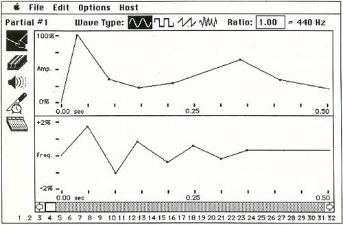
In 1975, the 16-bit Alto, which operated at a frequency of 5.88 MHz and possessed 128 Kbytes of RAM, already had some music software. In particular, for this computer there was a program TWANG , developed by Ted Kaehler (Ted Kaehler) in the Smalltalk language. In graphic form, quite in the spirit of modern musical MIDI editors, a stream of note events was demonstrated that could be added using the mouse or from the keyboard of an electronic organ. The sound was generated in real time by the method of FM synthesis, and each timbre parameter presented in the form of a graph could be adjusted, again, with the mouse. Drawing user envelopes with an arbitrary number of segments, as well as a visual representation of all the parameters of FM synthesis on a single graphic can not always be found even in modern software synthesizers.

View and edit note events in TWANG
FM synthesis was discovered in the late 60s by musician and scholar John Chowning from Stanford University during his experiments with one of the early MUSIC N audio languages N. Chowning noted that when using the usual vibrato effect (which is a periodic change in pitch) on sufficiently high frequency, the timbre of the modulated signal begins to change significantly. From the point of view of the listener, the greatest interest is not a static spectrum, but its various modifications that unfold in time. In this sense, FM synthesis has great potential with modest computational requirements, since, by controlling the amplitude and frequency of the modulator, it is easy to dynamically influence the spectrum of the carrier signal.
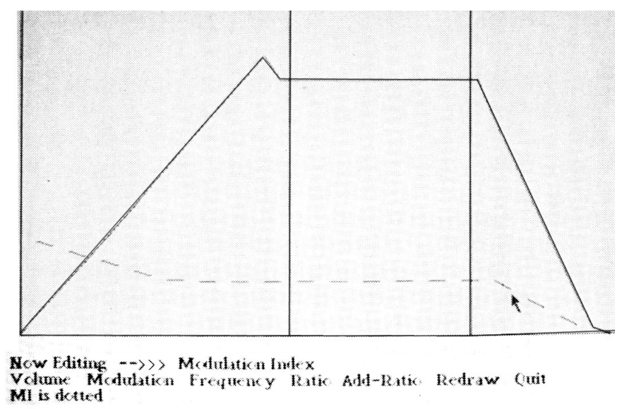
Editing FM synthesis parameters in TWANG
By the way, thanks to the funds obtained by Stanford University from the sale of the license for FM synthesis to Yamaha in the early 70s, the University established the CCRMA (Center for Computer Research in Music and Acoustics) research center. Many important results in the field of sound synthesis methods are associated with the name of this center.
Known parameters of FM-synthesis, implemented on Xerox Alto:
It is noteworthy that no special equipment, other than a DAC, was used to work with sound in Alto. FM synthesis was implemented in software and was performed simultaneously with GUI processing and other tasks. How, then, was the modest computer able to cope with real-time synthesis? The fact is that in Alto, the programmer was allowed to update the microcode right while the computer was running. Work at the microcode level was widely used by Xerox PARC developers to control external devices, as well as to virtualize a set of instructions and create problem-oriented commands, for example, for working with graphics. In the computer there was also hardware support for cooperative multitasking for the processes that performed the microcode.
An example of working in TWANG
To output the sound in TWANG, special instructions were used. The appropriate microcode for implementing FM synthesis was added by Steve Saunders. In his implementation, he managed to do without multiplication operations using two simple techniques : by replacing the sine with a triangular signal in the modulator, and also using the trigonometric identity sin (x + a) + sin (x - a) = 2 * cos (a) * sin (x) for amplitude control. It is interesting to note that Yamaha later, in its own way, got rid of multiplication operations in its FM chips using log and exp tables .
TWANG sound sample
The TWANG program has not received further development. Saunders in the early 80s had a hand in the development of the Atari Amy sound chip. This chip was a fairly powerful additive synthesizer for microcomputers, leading the sound quality of typical sound generators of the time, but Atari’s turmoil prevented Amy from seeing the light.
At once I will clarify what will be discussed later on phase (PM), and not frequency modulation, although the second naming will be used. It is the phase modulation option implemented by Yamaha in their FM synthesizers.
In the examples of this section, it will be convenient to use the form of the description of the sine wave generator in the form of an object that stores the current phase and has the next method for issuing the next sample. The parameter t is not explicitly used here, as was the case with the DTMF signals, and the phase value changes within the period of the sin function.
In FM synthesis, oscillators are combined in various configurations based on the following basic compounds: serial, parallel (additive synthesis), and with feedback. Even using only two oscillators connected in series, you can get quite complex timbres. In this case, the output of one of the oscillators is fed to the input of the phase offset of the other oscillator. From the point of view of creating timbres, such a variant of connection can be approximately considered as a pair of oscillator-filter in an analog synthesizer. Below is an example of the implementation of a serial connection for the synthesis of the simplest tone of a bell.
Source
Sound
In this example, the osc oscillator om ("modulator") controls the sound of the main oscillator oc ("carrier"). The following parameters are responsible for the characteristic timbre of the bell:
It is quite difficult to give a short recipe on the choice of parameters for synthesizing FM timbres. Theoretical information on this subject can be found in the book FM Theory & Applications . But, often, intuition and practice are more important. In general, in sound design, the basic approach is to decompose a complex timbre, dividing it into separate layers and elements so that you can work on them almost independently.
For convenient work with control signals that dynamically change, as, for example, this happens with the modulator amplitude in this case, it is useful to implement an envelope generator. Its code is shown below.
The envelope is determined using an array of linear segments. The x coordinate usually sets the time, and the y coordinate can be interpreted differently, for example, as amplitude or frequency.
The following example on the topic of FM synthesis and envelopes is related to the simulation of percussions. Here the timbres of a bass drum (kick) and a snare drum (snare) are implemented. Note that the synthesis code of the working drum uses a combination of oscillators with feedback (variable fb). The use of feedback in FM synthesis (it was an invention of Yamaha) allows you to create a large variety of timbres by simple efforts. With its help, it is possible to generate noise, as in this case, as well as creating sawtooth and rectangular sound waves. Numerous envelope generators are used in this example, not only to control the amplitude, but also the frequency of the oscillators.
Source
Sound
In general, the most realistic timbres are obtained in FM synthesis using 6 or more oscillators, but operating with such configurations lies beyond the capabilities of ordinary electronic musicians, therefore at present this type of synthesis is most often combined with other approaches.
In the late 70s, special speech synthesis chips began to gain popularity. Among the first was the chip TMS5100, which was used in the popular children's toy Speak & Spell. The development of this microcircuit demanded remarkable efforts from Texas Instruments engineers and its appearance is considered an important milestone in the development of processors for digital signal processing. Against this background, the story of SAM (Software Automatic Mouth) seems to be especially surprising - a fully software speech synthesizer, which was born back in 1979 and by the early 80s was implemented on the simplest 8-bit microcomputers by Apple, Atari and Commodore.

SAM Advertising
SAM was a set of programs without any graphical interface. With the help of these programs, it was possible to immediately translate arbitrary text to speech or, using the phonetic alphabet, to preliminarily describe in detail the method of sounding texts with a synthesizer. The clarity of phrases, in my opinion, at SAM is not inferior to chips from Texas Instruments. Moreover, in the version of formant synthesis implemented in SAM, it is possible on the fly to change the timbre and intonation of the voice with which user phrases are pronounced.
What is formant synthesis? The most thorough approach to the synthesis of voice are solutions based on physical modeling, differing in both computational complexity and complexity of customization. A simpler way is to use tone and noise generators, which are processed by a set of band-pass filters that simulate formants (peaks in the signal spectrum that determine speech sounds). In the case of Speak & Spell, ready-made phrases were coded based on linear prediction (LPC). The corresponding parameters determine the operation of the tone and noise generator, as well as the 10th order digital filter that is common to them.
The calculation of the next value at the output of the Speak & Spell filter required 20 multiplication operations, which was clearly beyond the capabilities of microcomputers of that time. What is the trick used by the creators of SAM? Apparently, this question did not give rest to researchers for many years, until finally, in the mid-2000s, the SAM code for the Commodore C64 microcomputer was not disassembled and translated into C language .
As it turned out, the implementation of speech synthesis in SAM did without a single multiplication operation at all. To generate formants, only the generators of a sine wave and a square wave appear in the code. Generally speaking, there is a synthesis of sinusoidal waves, in which the formation of formants is simply replaced by sinusoids at the corresponding frequencies, but this option is not distinguished by intelligibility of speech. SAM's approach is different. Its origins are in the theory of wavelets and granular synthesis . There are many variations of this approach, but their main feature is the imitation of the effect of the band-pass filter. Since the “filter” is fictitious, it is impossible to send any third-party signal to it. Instead of the complex implementation of real band-pass filters, formant synthesis is carried out at the level of generation of “bursts” or “granules” of waveforms. Similarly, the filters in the Casio CZ, Roland MT-32 and Yamaha FS1r synthesizers are simulated. One of the most well-known varieties of this approach is FOF (Formant Wave Function), which has successfully proved itself in the synthesis of singing .
Beg a small digression. A good third of the film “Steve Jobs” (2015) is devoted to an overly dramatic depiction of events related to the problems of launching a speech synthesizer during the presentation of the first Macintosh, which took place in 1984. You can learn how things were in reality from the memories of Andy Hertzfeld, one of the key Apple developers at the time. Steve Jobs was a connoisseur of music, both classical and popular. Obviously, for this reason, as well as impressed by the advanced computers of the 70s Xerox, the sound subsystem of a good (at that time) quality was implemented in the Macintosh: mono, 22 kHz, 8 bits. It was important for Jobs that at the presentation the computer would lose the solemn melody from the Chariots of Fire by Vangelis. Alas, time was running out, and Herzfeld managed to synthesize timbres only at the level of DTMF-signals, which we implemented in the first example. In this situation, the Macintosh team was rescued by Mark Barton, none other than the author of SAM. Of course, Jobs was delighted with the idea that the computer would introduce itself. So it happened. That's just “Chariots of Fire” was launched during a presentation from a CD player, and the 128K computer model had to be secretly replaced for 512K for the sake of a speech synthesizer, which was still in development. However, this is another story.
The SAM version of Mac for Macintosh called MacinTalk, in contrast to the microcomputer options, generated a higher quality 8-bit sound. SAM, the maker of SoftVoice, eventually released versions of speech synthesizers for Amiga and Windows. To date, apparently, SoftVoice no longer exists, but the popularity of the restored SAM source code is growing among developers of embedded systems who want to implement simple speech synthesis on resource-limited microcontrollers.
From studying the SAM code, it is clear that this speech synthesizer has only 4 oscillators:
2 sine wave generators, a square wave generator (square wave), as well as a pulse generator that simulates the operation of the vocal cords. The parameters of these oscillators are encoded in a stream of frames, which are updated with a certain frequency corresponding to the speed of "pronouncing" phrases.
The meander generator can be implemented in the most primitive way using the ternary conditional operator (in C syntax it looks like this: phase <0.5? 1: -1 ). This option, generally speaking, suffers from one very common drawback from the world of digital signal processing: frequency overlaying (aliasing). An ideal meander has an infinite spectrum, but sound waves should not contain frequencies greater than or equal to half the sampling frequency (Kotelnikov's theorem), otherwise we risk getting “dirt” that is quite audible in the spectrum. An entire book can be devoted to different ways to achieve the correct signal spectrum for the simplest “square” or “saw”. One of the simple tricks is using FM synthesis with feedback. Now, the “wrong” way will be enough for us. I also put the word “wrong” in quotes because the music synthesis algorithms are not exactly the same as regular digital signal processing. In music, the result is important from an aesthetic point of view, even if it was not obtained “according to science”. In the case of SAM, this is also true, since this voice synthesizer was created for sound output by 8-bit microcomputers.
Source
Frames
Sound
A key in the work of SAM is a pulse generator (its index in the array of arrays is zero), imitating the work of the vocal cords, although it does not produce sound by itself. The result of his work is the zeroing of the phases of the other oscillators with a frequency corresponding to the chosen type of voice. This method of synthesizing formants by resetting the oscillator-carrier oscillator-modulator phase is known in the world of analog synthesizers as hard sync .
Example of “tight” synchronization of a sine wave in SAM
Initially, I wanted to implement the synthesis of the phrase My name is Sam, but then the hissing and whistling consonants would have to be supported with the help of pre-recorded sound bites (as was done in the original program). Therefore, I stopped only on the part of My name. A more complete solution would be to support noise generators with various parameters.
One of the first developers of commercial music software for the Apple Macintosh 128K computer was Peter Gotcher and Evan Brooks, friends who played on the same student team and were fond of both music and programming. In 1986, Gotcher and Brooks released a program with a talking name SoftSynth. Yesterday’s students implemented high-grade additive synthesis with the following parameters:
SoftSynth had advanced tools for editing synthesis parameters, as well as their visualization (including in the form of a 3d spectrogram - in the spirit of the famous Fairlight CMI synthesizer).
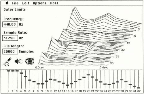
SoftSynth 3d spectrogram
Editing oscillator envelopes in SoftSynth
It seems surprising that the possibilities of the ancient Macintosh were enough to implement such a synthesis. The secret is simple: the process of creating sound in SoftSynth did not occur in real time, but by clicking on a special icon. Typing a typical short sample took no more than a few seconds. SoftSynth can be attributed to the now forgotten class of program-generator samples. Distracting, you can remember Oleg Sharonov's Orangator, a popular program from the same class in the late 90s.

Orangator Interface
By the mid-80s, the popularity of hardware samplers (such as, for example, E-MU Emulator, released in 1982) had grown enormously, and the program, which made it possible to synthesize samples from scratch for later loading them into the memory of hardware tools, was in demand by musicians.
But how did young developers, such as Gotscher and Brooks, receive information related to the principles of computer sound in the early 80s? By that time there were already at least three important sources on this topic:
Obviously, under the influence of both modular analog synthesizers and the graphic notation MUSIC V from Matthews, an interface was developed for another, quite advanced for its time, musical program for the Macintosh computer from the Gotscher and Brooks team. This program was called Turbosynth (1988). Turbosynth, like SoftSynth, is a sample generator. The user is provided with a palette of sound modules, copies of which can be transferred with the mouse to the workspace and, further, connected to taste with virtual “wires”. The program has implemented a large number of modules:

Connecting modules in Turbosynth
In general, working with Turbosynth differs little from later visual music programming environments (Kyma, Max / MSP, Pure Data, Reaktor). It is known that experimenter musician Trent Reznor (Trent Reznor, Nine Inch Nails) widely used TurboSynth in 1993, during the recording of the album Mr. Self Destruct.
What was the fate of Gotcher and Brooks? They became known as the creators of the Pro Tools software and hardware system, which is still used in many professional recording studios.
I now propose to consider another example of additive synthesis called the Arpeggio Rissa. The author of this simple but interesting sound algorithm is Jean-Claude Risset, one of the pioneers of computer music. In the implementation of the Arpeggio Risse, 63 sine wave generators are used, the frequencies of which are set so that the effect of the beats leads to sound with a constantly changing timbre.
Source
The sound of
the Arpeggio Riss is the simplest example of a process music. There is no division into instruments and notes. A single algorithm spawns the entire piece of music.
The following example is less related to sound synthesis. The implementation of the sound algorithm using the description of blocks and the links between them can be represented both in text (MUSIC N) and in graphical (TurboSynth) form. In both cases, an approach is used in which calculations are controlled by data flows (dataflow). This approach is known in many areas of computer science: compilation theory, processor architectures, distributed systems, etc. Let's try to create a simple dataflow model in text form. We will use blocks (box), which are engaged in calculations, and also provide the ability to randomly connect blocks with wires (wire). Programs such as Pure Data and Max / MSP use two types of links:
For simplicity, we restrict ourselves to synchronous connections. More specifically, to start the calculation inside the block, we will require the following conditions:
So, the unit has a number of input and output ports. In the following implementation, it is prohibited to connect several wires to one input port, but it is allowed to stretch several wires from a single output port of the unit. For this reason, in the block object, each element of the array of output ports is itself an array of connected consumer blocks.
To describe the calculations, it is enough to specify the list of blocks (“schedule”) and determine the appropriate links. Pay attention to the compute function. She simply tries to run the calculations for each block specified in the schedule. The order of the blocks here does not matter for the correctness of the calculations. However, this sequence affects the efficiency of the calculations. It is desirable that the blocks that produce values precede the blocks that consume these values. Arrange the schedule accordingly using the topological sorting algorithm . The fact that any of the blocks, in accordance with the rule of readiness of input and output data, can independently start calculations, makes it possible to easily parallelize the operation of the graph of the sound algorithm.
Now let's try to put into practice the above. Let us create the simplest sound of a siren.
Source
Sound
In this example, the following block types are used:

Graphic representation of the implementation of the "siren"
One may ask why the Clip block was required. With it, we achieve the simplest effect of sound distortion. Instead of a “sterile” sinusoid, we got a signal close to the meander.
Graphic representation of this simple sound algorithm turned out to be more vivid than its text recording. But it is rather a lack of a specific implementation. In general, the text form usually wins over the graphical variant when using a sufficiently large number of blocks and links. The informal “Deutsch limit” , in particular, features 50 blocks as the corresponding upper bound.
Go to the second part
Go to the second part
Introduction
In the second half of the 90s, I enthusiastically got acquainted with computer music on a PC and tried to compose my compositions in popular then tracker programs, such as Fast Tracker II and EdLib. But the greatest impression on me in those days was the Csound audio language, which I learned about, thanks to a 1998 article from Computerra magazine . To work with Csound you need only a text editor. The speed of the computer, the presence of libraries of sampled sounds or the quality of the sound card did not matter. It was a software synthesis of sound in its purest form.
')
On modern personal computers, it is not difficult to implement the once-impressive musical examples for Csound in real time. Today, specialized hardware solutions for problems of sound synthesis are used by musicians less and less, and audio plugs have become most popular. So the matter, of course, was not always the case. What were the first attempts to create software synthesis on early personal computers? What were these computers? Finally, what are the details of the implementation of the early methods of program synthesis? I will try to answer these questions further.
Practice
In my opinion, teaching in the historical context has many advantages and therefore, along with the description of the cases of bygone days, I wanted to encourage readers, not alien to programming, to practical sound design. I will not go into the theory, because I see it as my task to develop an initial and intuitive idea for interested readers about how synthesizers are programmed. For this reason, the examples that will be shown below are implemented without typical tricks and tricks familiar to experienced developers.
We will work in the spirit of the pioneers of computer music of the 60s, who used in their research the MUSIC N audio language series developed by Max Mathews. Csound, which was discussed above, is one of the many descendants of MUSIC N. Of course, we have certain advantages over the pioneers: you do not need to wait for the code to be compiled for long hours, you do not need to write the result to magnetic tape, and then go with it to another city in order to transfer the received data to sound on another computer.
Sound synthesis examples will be given in Python. One of the important advantages of this language is the similarity of its syntax with pseudocode, the reading of which should not cause particular difficulties even for readers who are not familiar with Python. The programs proposed in the article serve purely illustrative purposes and are intended to encourage the reader to experiment with sound algorithms. Each example is a separate program for versions 2 and 3 of the language and depends only on the standard libraries. Running examples ends with the formation of a wav file. Using PyPy will speed up the calculations several times.
To save the result in a wav-file, I use the standard wave module. All further examples are preceded by the code shown below.
SR = 44100 # 16- # SR wav- def write_wave(filename, samples): f = wave.open(filename, "w") f.setparams((1, 2, SR, len(samples), "NONE", "")) f.writeframes(b"".join( [struct.pack('<h', round(x * 32767)) for x in samples])) f.close() # def sec(x): return SR * x Here is a simple example in which only pairs of sinusoids are used.
# , , bank def sines(bank, t): mix = 0 for f in bank: mix += math.sin(2 * math.pi * f * t / SR) return mix # DTMF- 1-9 DTMF = [ [697, 1209], [697, 1336], [697, 1477], [770, 1209], [770, 1336], [770, 1477], [852, 1209], [852, 1336], [852, 1477] ] samples = [] # for d in [3, 1, 1, 5, 5, 5, 2, 3, 6, 8]: for t in range(int(sec(0.05))): samples.append(0.5 * sines(DTMF[d - 1], t)) for t in range(int(sec(0.05))): samples.append(0) write_wave("dtmf.wav", samples) Source
Sound
Here the tone dial sound is generated for the fictitious phone number 3115552368. The digits of the DTMF number are encoded with pairs of sinusoids whose frequencies are specified in the DTMF array. Pay attention to the characteristic clicks in the sound, which are the result of sudden amplitude drops. To get rid of such clicks, you can use the amplitude envelope or low-pass filter. The use of envelopes and filters will be described in more detail below.
TWANG
And they, in fact, showed me three things. But I was so impressed with the first of these things that I did not pay attention to the rest. Among other things, they showed me object-oriented programming, which I did not notice. They also showed me a computer network ... in which more than a hundred Alto computers were connected, there was email, etc., etc. I did not notice all this, as I was completely blinded by the first thing that was shown to me - a graphical user interface.So, after a while, Steve Jobs recalled his visit to the Xerox PARC research center in 1979. Computer Xerox Alto, which was created in 1973, in many respects anticipated the appearance of personal computers in the next decades. The author of the Alto concept is the scholar Alan Kay (Alan Kay), who is no stranger to music: in his youth he managed to visit a jazz guitarist, and in his mature years he mastered a church organ. Perhaps for this reason, Alto had not only outstanding graphics capabilities for its time, but also good sound support.
In 1975, the 16-bit Alto, which operated at a frequency of 5.88 MHz and possessed 128 Kbytes of RAM, already had some music software. In particular, for this computer there was a program TWANG , developed by Ted Kaehler (Ted Kaehler) in the Smalltalk language. In graphic form, quite in the spirit of modern musical MIDI editors, a stream of note events was demonstrated that could be added using the mouse or from the keyboard of an electronic organ. The sound was generated in real time by the method of FM synthesis, and each timbre parameter presented in the form of a graph could be adjusted, again, with the mouse. Drawing user envelopes with an arbitrary number of segments, as well as a visual representation of all the parameters of FM synthesis on a single graphic can not always be found even in modern software synthesizers.
View and edit note events in TWANG
FM synthesis was discovered in the late 60s by musician and scholar John Chowning from Stanford University during his experiments with one of the early MUSIC N audio languages N. Chowning noted that when using the usual vibrato effect (which is a periodic change in pitch) on sufficiently high frequency, the timbre of the modulated signal begins to change significantly. From the point of view of the listener, the greatest interest is not a static spectrum, but its various modifications that unfold in time. In this sense, FM synthesis has great potential with modest computational requirements, since, by controlling the amplitude and frequency of the modulator, it is easy to dynamically influence the spectrum of the carrier signal.
Editing FM synthesis parameters in TWANG
By the way, thanks to the funds obtained by Stanford University from the sale of the license for FM synthesis to Yamaha in the early 70s, the University established the CCRMA (Center for Computer Research in Music and Acoustics) research center. Many important results in the field of sound synthesis methods are associated with the name of this center.
Known parameters of FM-synthesis, implemented on Xerox Alto:
- 5 votes (2 oscillators each) working in real time
- 12-bit samples with a sampling frequency of 13.7 kHz,
- Update the parameters of voices at 60 Hz.
It is noteworthy that no special equipment, other than a DAC, was used to work with sound in Alto. FM synthesis was implemented in software and was performed simultaneously with GUI processing and other tasks. How, then, was the modest computer able to cope with real-time synthesis? The fact is that in Alto, the programmer was allowed to update the microcode right while the computer was running. Work at the microcode level was widely used by Xerox PARC developers to control external devices, as well as to virtualize a set of instructions and create problem-oriented commands, for example, for working with graphics. In the computer there was also hardware support for cooperative multitasking for the processes that performed the microcode.
An example of working in TWANG
To output the sound in TWANG, special instructions were used. The appropriate microcode for implementing FM synthesis was added by Steve Saunders. In his implementation, he managed to do without multiplication operations using two simple techniques : by replacing the sine with a triangular signal in the modulator, and also using the trigonometric identity sin (x + a) + sin (x - a) = 2 * cos (a) * sin (x) for amplitude control. It is interesting to note that Yamaha later, in its own way, got rid of multiplication operations in its FM chips using log and exp tables .
TWANG sound sample
The TWANG program has not received further development. Saunders in the early 80s had a hand in the development of the Atari Amy sound chip. This chip was a fairly powerful additive synthesizer for microcomputers, leading the sound quality of typical sound generators of the time, but Atari’s turmoil prevented Amy from seeing the light.
Practice
At once I will clarify what will be discussed later on phase (PM), and not frequency modulation, although the second naming will be used. It is the phase modulation option implemented by Yamaha in their FM synthesizers.
In the examples of this section, it will be convenient to use the form of the description of the sine wave generator in the form of an object that stores the current phase and has the next method for issuing the next sample. The parameter t is not explicitly used here, as was the case with the DTMF signals, and the phase value changes within the period of the sin function.
class Sine: def __init__(self): self.phase = 0 # freq pm, # , , # phase, def next(self, freq, pm=0): s = math.sin(self.phase + pm) self.phase = (self.phase + 2 * math.pi * freq / SR) % (2 * math.pi) return s In FM synthesis, oscillators are combined in various configurations based on the following basic compounds: serial, parallel (additive synthesis), and with feedback. Even using only two oscillators connected in series, you can get quite complex timbres. In this case, the output of one of the oscillators is fed to the input of the phase offset of the other oscillator. From the point of view of creating timbres, such a variant of connection can be approximately considered as a pair of oscillator-filter in an analog synthesizer. Below is an example of the implementation of a serial connection for the synthesis of the simplest tone of a bell.
# FM- # y(t) = Ac * sin(2 * PI * fc * t + Am * sin(2 * PI * fm * t)) oc = Sine() om = Sine() samples = [] for t in range(int(sec(1))): env = 1 - t / SR samples.append(0.5 * oc.next(80, 3 * env * om.next(450))) write_wave("bell.wav", samples) Source
Sound
In this example, the osc oscillator om ("modulator") controls the sound of the main oscillator oc ("carrier"). The following parameters are responsible for the characteristic timbre of the bell:
- the ratio of the modulator and carrier frequencies, creating non-harmonic overtones,
- linear attenuation of the amplitude of the modulator (3 * env), which introduces the desired dynamics in the spectral composition.
It is quite difficult to give a short recipe on the choice of parameters for synthesizing FM timbres. Theoretical information on this subject can be found in the book FM Theory & Applications . But, often, intuition and practice are more important. In general, in sound design, the basic approach is to decompose a complex timbre, dividing it into separate layers and elements so that you can work on them almost independently.
For convenient work with control signals that dynamically change, as, for example, this happens with the modulator amplitude in this case, it is useful to implement an envelope generator. Its code is shown below.
# - , def linear_env(segs, t): x0 = 0 y0 = 0 for x1, y1 in segs: if t < x1: return y0 + (t - x0) * ((y1 - y0) / (x1 - x0)) x0, y0 = x1, y1 return y0 class Env: def __init__(self, segs): self.segs = segs self.phase = 0 def next(self, scale=1): s = linear_env(self.segs, self.phase) self.phase += scale / SR return s The envelope is determined using an array of linear segments. The x coordinate usually sets the time, and the y coordinate can be interpreted differently, for example, as amplitude or frequency.
The following example on the topic of FM synthesis and envelopes is related to the simulation of percussions. Here the timbres of a bass drum (kick) and a snare drum (snare) are implemented. Note that the synthesis code of the working drum uses a combination of oscillators with feedback (variable fb). The use of feedback in FM synthesis (it was an invention of Yamaha) allows you to create a large variety of timbres by simple efforts. With its help, it is possible to generate noise, as in this case, as well as creating sawtooth and rectangular sound waves. Numerous envelope generators are used in this example, not only to control the amplitude, but also the frequency of the oscillators.
def kick(samples, dur): freq = 100 o1 = Sine() o2 = Sine() e1 = Env([(0, 1), (0.03, 1), (1, 0)]) e2 = Env([(0, 1), (0.01, 0)]) for t in range(int(sec(dur))): o = o1.next(freq * e1.next(2.5), 14 * e2.next() * o2.next(freq)) samples.append(0.5 * o) def snare(samples, dur): freq = 100 o1 = Sine() o2 = Sine() e1 = Env([(0, 1), (0.2, 0.2), (0.4, 0)]) e2 = Env([(0, 1), (0.17, 0)]) e3 = Env([(0, 1), (0.005, 0.15), (1, 0)]) fb = 0 for t in range(int(sec(dur))): fb = e2.next() * o1.next(freq, 1024 * fb) samples.append(0.5 * o2.next(e1.next() * freq * 2.5, 5.3 * e3.next() * fb)) samples = [] for i in range(4): kick(samples, 0.25) kick(samples, 0.25) snare(samples, 0.5) write_wave("drums.wav", samples) Source
Sound
In general, the most realistic timbres are obtained in FM synthesis using 6 or more oscillators, but operating with such configurations lies beyond the capabilities of ordinary electronic musicians, therefore at present this type of synthesis is most often combined with other approaches.
SAM
In the late 70s, special speech synthesis chips began to gain popularity. Among the first was the chip TMS5100, which was used in the popular children's toy Speak & Spell. The development of this microcircuit demanded remarkable efforts from Texas Instruments engineers and its appearance is considered an important milestone in the development of processors for digital signal processing. Against this background, the story of SAM (Software Automatic Mouth) seems to be especially surprising - a fully software speech synthesizer, which was born back in 1979 and by the early 80s was implemented on the simplest 8-bit microcomputers by Apple, Atari and Commodore.
SAM Advertising
SAM was a set of programs without any graphical interface. With the help of these programs, it was possible to immediately translate arbitrary text to speech or, using the phonetic alphabet, to preliminarily describe in detail the method of sounding texts with a synthesizer. The clarity of phrases, in my opinion, at SAM is not inferior to chips from Texas Instruments. Moreover, in the version of formant synthesis implemented in SAM, it is possible on the fly to change the timbre and intonation of the voice with which user phrases are pronounced.
What is formant synthesis? The most thorough approach to the synthesis of voice are solutions based on physical modeling, differing in both computational complexity and complexity of customization. A simpler way is to use tone and noise generators, which are processed by a set of band-pass filters that simulate formants (peaks in the signal spectrum that determine speech sounds). In the case of Speak & Spell, ready-made phrases were coded based on linear prediction (LPC). The corresponding parameters determine the operation of the tone and noise generator, as well as the 10th order digital filter that is common to them.
The calculation of the next value at the output of the Speak & Spell filter required 20 multiplication operations, which was clearly beyond the capabilities of microcomputers of that time. What is the trick used by the creators of SAM? Apparently, this question did not give rest to researchers for many years, until finally, in the mid-2000s, the SAM code for the Commodore C64 microcomputer was not disassembled and translated into C language .
As it turned out, the implementation of speech synthesis in SAM did without a single multiplication operation at all. To generate formants, only the generators of a sine wave and a square wave appear in the code. Generally speaking, there is a synthesis of sinusoidal waves, in which the formation of formants is simply replaced by sinusoids at the corresponding frequencies, but this option is not distinguished by intelligibility of speech. SAM's approach is different. Its origins are in the theory of wavelets and granular synthesis . There are many variations of this approach, but their main feature is the imitation of the effect of the band-pass filter. Since the “filter” is fictitious, it is impossible to send any third-party signal to it. Instead of the complex implementation of real band-pass filters, formant synthesis is carried out at the level of generation of “bursts” or “granules” of waveforms. Similarly, the filters in the Casio CZ, Roland MT-32 and Yamaha FS1r synthesizers are simulated. One of the most well-known varieties of this approach is FOF (Formant Wave Function), which has successfully proved itself in the synthesis of singing .
Beg a small digression. A good third of the film “Steve Jobs” (2015) is devoted to an overly dramatic depiction of events related to the problems of launching a speech synthesizer during the presentation of the first Macintosh, which took place in 1984. You can learn how things were in reality from the memories of Andy Hertzfeld, one of the key Apple developers at the time. Steve Jobs was a connoisseur of music, both classical and popular. Obviously, for this reason, as well as impressed by the advanced computers of the 70s Xerox, the sound subsystem of a good (at that time) quality was implemented in the Macintosh: mono, 22 kHz, 8 bits. It was important for Jobs that at the presentation the computer would lose the solemn melody from the Chariots of Fire by Vangelis. Alas, time was running out, and Herzfeld managed to synthesize timbres only at the level of DTMF-signals, which we implemented in the first example. In this situation, the Macintosh team was rescued by Mark Barton, none other than the author of SAM. Of course, Jobs was delighted with the idea that the computer would introduce itself. So it happened. That's just “Chariots of Fire” was launched during a presentation from a CD player, and the 128K computer model had to be secretly replaced for 512K for the sake of a speech synthesizer, which was still in development. However, this is another story.
The SAM version of Mac for Macintosh called MacinTalk, in contrast to the microcomputer options, generated a higher quality 8-bit sound. SAM, the maker of SoftVoice, eventually released versions of speech synthesizers for Amiga and Windows. To date, apparently, SoftVoice no longer exists, but the popularity of the restored SAM source code is growing among developers of embedded systems who want to implement simple speech synthesis on resource-limited microcontrollers.
Practice
From studying the SAM code, it is clear that this speech synthesizer has only 4 oscillators:
2 sine wave generators, a square wave generator (square wave), as well as a pulse generator that simulates the operation of the vocal cords. The parameters of these oscillators are encoded in a stream of frames, which are updated with a certain frequency corresponding to the speed of "pronouncing" phrases.
The meander generator can be implemented in the most primitive way using the ternary conditional operator (in C syntax it looks like this: phase <0.5? 1: -1 ). This option, generally speaking, suffers from one very common drawback from the world of digital signal processing: frequency overlaying (aliasing). An ideal meander has an infinite spectrum, but sound waves should not contain frequencies greater than or equal to half the sampling frequency (Kotelnikov's theorem), otherwise we risk getting “dirt” that is quite audible in the spectrum. An entire book can be devoted to different ways to achieve the correct signal spectrum for the simplest “square” or “saw”. One of the simple tricks is using FM synthesis with feedback. Now, the “wrong” way will be enough for us. I also put the word “wrong” in quotes because the music synthesis algorithms are not exactly the same as regular digital signal processing. In music, the result is important from an aesthetic point of view, even if it was not obtained “according to science”. In the case of SAM, this is also true, since this voice synthesizer was created for sound output by 8-bit microcomputers.
class Sam: def __init__(self): self.phases = [0, 0, 0, 0] # frame , voice def next(self, frame, voice): flags, ampl1, freq1, ampl2, freq2, ampl3, freq3, pitch = frame mix = ampl1 * math.sin(self.phases[1]) + ampl2 * math.sin(self.phases[2]) mix += ampl3 * (1 if self.phases[3] < 0.5 else -1) self.phases[1] = (self.phases[1] + 2 * math.pi * freq1 / SR) % (2 * math.pi) self.phases[2] = (self.phases[2] + 2 * math.pi * freq2 / SR) % (2 * math.pi) self.phases[3] = (self.phases[3] + freq3 / SR) % 1 self.phases[0] += 1 if self.phases[0] > pitch * voice * SR: self.phases = [0, 0, 0, 0] return 0.5 * mix # SAM 64 COEFFS = [1, 0.1, 27, 0.1, 27, 0.1, 27, 0.00001] # def parse(frames): frames = [[int(y) * COEFFS[i] for i, y in enumerate(x.split())] \ for x in frames.strip().split("\n")] return frames # sam.txt # https://github.com/s-macke/SAM -debug with open("sam.txt") as f: frames = parse(f.read()) s = Sam() samples = [] # " " for voice in range(25, 5, -2): for frame in frames: for t in range(int(sec(0.01))): samples.append(0.5 * s.next(frame, voice)) write_wave("sam.wav", samples) Source
Frames
Sound
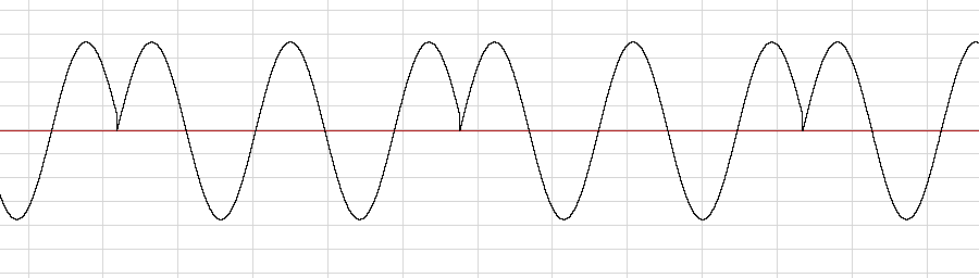
A key in the work of SAM is a pulse generator (its index in the array of arrays is zero), imitating the work of the vocal cords, although it does not produce sound by itself. The result of his work is the zeroing of the phases of the other oscillators with a frequency corresponding to the chosen type of voice. This method of synthesizing formants by resetting the oscillator-carrier oscillator-modulator phase is known in the world of analog synthesizers as hard sync .
Example of “tight” synchronization of a sine wave in SAM
Initially, I wanted to implement the synthesis of the phrase My name is Sam, but then the hissing and whistling consonants would have to be supported with the help of pre-recorded sound bites (as was done in the original program). Therefore, I stopped only on the part of My name. A more complete solution would be to support noise generators with various parameters.
SoftSynth and TurboSynth
One of the first developers of commercial music software for the Apple Macintosh 128K computer was Peter Gotcher and Evan Brooks, friends who played on the same student team and were fond of both music and programming. In 1986, Gotcher and Brooks released a program with a talking name SoftSynth. Yesterday’s students implemented high-grade additive synthesis with the following parameters:
- 32 (, «», «» 3 ),
- , 40 .
SoftSynth had advanced tools for editing synthesis parameters, as well as their visualization (including in the form of a 3d spectrogram - in the spirit of the famous Fairlight CMI synthesizer).
SoftSynth 3d spectrogram
Editing oscillator envelopes in SoftSynth
It seems surprising that the possibilities of the ancient Macintosh were enough to implement such a synthesis. The secret is simple: the process of creating sound in SoftSynth did not occur in real time, but by clicking on a special icon. Typing a typical short sample took no more than a few seconds. SoftSynth can be attributed to the now forgotten class of program-generator samples. Distracting, you can remember Oleg Sharonov's Orangator, a popular program from the same class in the late 90s.
Orangator Interface
By the mid-80s, the popularity of hardware samplers (such as, for example, E-MU Emulator, released in 1982) had grown enormously, and the program, which made it possible to synthesize samples from scratch for later loading them into the memory of hardware tools, was in demand by musicians.
But how did young developers, such as Gotscher and Brooks, receive information related to the principles of computer sound in the early 80s? By that time there were already at least three important sources on this topic:
- The Technology of Computer Music (1969) by Max Mathews (Max Mathews), which described the audio language MUSIC V and the simplest methods of synthesis.
- Musical Applications of Microprocessors (1980) (Hal Chamberlin). , . , .
- Computer Music Journal, 1977 , , .
Obviously, under the influence of both modular analog synthesizers and the graphic notation MUSIC V from Matthews, an interface was developed for another, quite advanced for its time, musical program for the Macintosh computer from the Gotscher and Brooks team. This program was called Turbosynth (1988). Turbosynth, like SoftSynth, is a sample generator. The user is provided with a palette of sound modules, copies of which can be transferred with the mouse to the workspace and, further, connected to taste with virtual “wires”. The program has implemented a large number of modules:
- an oscillator with a choice of different waveforms, the ability to morph these shapes using the time scale, as well as the ability to draw custom waveforms,
- sampler,
- noise generator
- c ,
- - ,
- ,
- ,
- ,
- AM-, FM- PM-,
- «» ,
- (waveshaper) ,
- .
Connecting modules in Turbosynth
In general, working with Turbosynth differs little from later visual music programming environments (Kyma, Max / MSP, Pure Data, Reaktor). It is known that experimenter musician Trent Reznor (Trent Reznor, Nine Inch Nails) widely used TurboSynth in 1993, during the recording of the album Mr. Self Destruct.
What was the fate of Gotcher and Brooks? They became known as the creators of the Pro Tools software and hardware system, which is still used in many professional recording studios.
Practice
I now propose to consider another example of additive synthesis called the Arpeggio Rissa. The author of this simple but interesting sound algorithm is Jean-Claude Risset, one of the pioneers of computer music. In the implementation of the Arpeggio Risse, 63 sine wave generators are used, the frequencies of which are set so that the effect of the beats leads to sound with a constantly changing timbre.
def sines(bank, t): mix = 0 for f in bank: mix += math.sin(2 * math.pi * f * t / SR) return mix # f = 96 i1 = 0.03 i2 = i1 * 2 i3 = i1 * 3 i4 = i1 * 4 risset = [] # 63 (9 * 7) risset for i in [f, f + i1, f + i2, f + i3, f + i4, f - i1, f - i2, f - i3, f - i4]: for j in [i, 5 * i, 6 * i, 7 * i, 8 * i, 9 * i, 10 * i]: risset.append(j) samples = [] for t in range(int(sec(20))): samples.append(0.01 * sines(risset, t)) write_wave("risset.wav", samples) Source
The sound of
the Arpeggio Riss is the simplest example of a process music. There is no division into instruments and notes. A single algorithm spawns the entire piece of music.
The following example is less related to sound synthesis. The implementation of the sound algorithm using the description of blocks and the links between them can be represented both in text (MUSIC N) and in graphical (TurboSynth) form. In both cases, an approach is used in which calculations are controlled by data flows (dataflow). This approach is known in many areas of computer science: compilation theory, processor architectures, distributed systems, etc. Let's try to create a simple dataflow model in text form. We will use blocks (box), which are engaged in calculations, and also provide the ability to randomly connect blocks with wires (wire). Programs such as Pure Data and Max / MSP use two types of links:
- asynchronous, for example, note events,
- synchronous, for working with audio signals.
For simplicity, we restrict ourselves to synchronous connections. More specifically, to start the calculation inside the block, we will require the following conditions:
- the input wires of the block contain ready data,
- block output wires are free to get new data.
So, the unit has a number of input and output ports. In the following implementation, it is prohibited to connect several wires to one input port, but it is allowed to stretch several wires from a single output port of the unit. For this reason, in the block object, each element of the array of output ports is itself an array of connected consumer blocks.
# def reset_ins(ins): for i, x in enumerate(ins): ins[i] = None # def is_ins_full(ins): for x in ins: if x is None: return False return True # def is_outs_empty(outs): for out in outs: for box, port in out: if box.ins[port] is not None: return False return True # . def send_to_outs(results, outs): for i, x in enumerate(results): for box, port in outs[i]: box.ins[port] = x class Box: # , op, # ins outs def __init__(self, op, ins, outs): self.ins = [None] * ins self.outs = [[] for i in range(outs)] self.op = op def compute(self): if is_ins_full(self.ins) and is_outs_empty(self.outs): send_to_outs(self.op(*self.ins), self.outs) reset_ins(self.ins) # port1 box1 port2 box2 def wire(box1, port1, box2, port2): box1.outs[port1].append((box2, port2)) def compute(schedule): for b in schedule: b.compute() To describe the calculations, it is enough to specify the list of blocks (“schedule”) and determine the appropriate links. Pay attention to the compute function. She simply tries to run the calculations for each block specified in the schedule. The order of the blocks here does not matter for the correctness of the calculations. However, this sequence affects the efficiency of the calculations. It is desirable that the blocks that produce values precede the blocks that consume these values. Arrange the schedule accordingly using the topological sorting algorithm . The fact that any of the blocks, in accordance with the rule of readiness of input and output data, can independently start calculations, makes it possible to easily parallelize the operation of the graph of the sound algorithm.
Now let's try to put into practice the above. Let us create the simplest sound of a siren.
# Sine def Osc(): o = Sine() return Box(lambda x, y: [o.next(x, y)], 2, 1) def Out(samples): def compute(x): samples.append(x) return [] return Box(compute, 1, 0) def clip(x, y): return -y if x < -y else y if x > y else x Const = lambda x: Box(lambda: [x], 0, 1) Mul = lambda: Box(lambda x, y: [x * y], 2, 1) Clip = lambda: Box(lambda x, y: [clip(x, y)], 2, 1) samples = [] patch = { "k1": Const(550), "k2": Const(50), "k3": Const(2), "k4": Const(0), "k5": Const(0.1), "k6": Const(1), "o1": Osc(), "o2": Osc(), "c1": Clip(), "m1": Mul(), "m2": Mul(), "out": Out(samples) } wire(patch["k3"], 0, patch["o1"], 0) wire(patch["k4"], 0, patch["o1"], 1) wire(patch["k2"], 0, patch["m1"], 0) wire(patch["o1"], 0, patch["m1"], 1) wire(patch["k1"], 0, patch["o2"], 0) wire(patch["m1"], 0, patch["o2"], 1) wire(patch["o2"], 0, patch["c1"], 0) wire(patch["k5"], 0, patch["c1"], 1) wire(patch["k6"], 0, patch["m2"], 0) wire(patch["c1"], 0, patch["m2"], 1) wire(patch["m2"], 0, patch["out"], 0) schedule = patch.values() while len(samples) < int(sec(2)): compute(schedule) write_wave("siren.wav", samples) Source
Sound
In this example, the following block types are used:
- Const, constant,
- Mul, multiplier,
- Osc, sine wave generator,
- Out, output samples to the output buffer,
- Clip, limiting the signal within the specified level.
Graphic representation of the implementation of the "siren"
One may ask why the Clip block was required. With it, we achieve the simplest effect of sound distortion. Instead of a “sterile” sinusoid, we got a signal close to the meander.
Graphic representation of this simple sound algorithm turned out to be more vivid than its text recording. But it is rather a lack of a specific implementation. In general, the text form usually wins over the graphical variant when using a sufficiently large number of blocks and links. The informal “Deutsch limit” , in particular, features 50 blocks as the corresponding upper bound.
Go to the second part
Source: https://habr.com/ru/post/348036/
All Articles