Convolutional neural network, part 2: training in the error back-propagation algorithm
In the first part , the structure, topology, activation functions and training set were considered. In this part I will try to explain how the convolutional neural network is trained.
At the initial stage, the neural network is untrained (unconfigured). In a general sense, learning is the sequential presentation of an image to the input of a neural network, from the training set, then the resulting answer is compared with the desired output, in our case it is 1 - the image represents a person, minus 1 - the image represents a background (not the person), the difference between the expected The answer and the result is the result of the error function (delta error). Then this delta needs to be extended to all connected neurons of the network.
Thus, the training of the neural network is reduced to minimizing the error function by adjusting the weights of the synaptic connections between neurons. The error function is the difference between the received answer and the desired one. For example, a face image was submitted to the input, suppose that the output of the neural network was 0.73, and the desired result is 1 (because the face image), we find that the network error is the difference, that is, 0.27. Then the weights of the output layer of the neurons are adjusted in accordance with the error. For neurons of the output layer, their actual and desired output values are known. Therefore, setting up link weights for such neurons is relatively simple. However, the setting is not so obvious for neurons of the previous layers. For a long time, the algorithm for propagating errors across hidden layers was not known.
For learning the described neural network, the backpropagation algorithm was used. This method of teaching a multilayer neural network is called the generalized delta rule. The method was proposed in 1986 by Rumelhart, McCleland and Williams. This marked a revival of interest in neural networks, which began to fade away in the early 70s. This algorithm is the first and the main practically applicable for training multilayer neural networks.
')
For the output layer, the adjustment of the weights is intuitive, but for the hidden layers there has been no known algorithm for a long time. The weights of the hidden neuron should vary in direct proportion to the error of those neurons with which the neuron is associated. That is why the reverse propagation of these errors through the network allows you to correctly adjust the weights of the connections between all layers. In this case, the magnitude of the error function is reduced and the network is trained.
The basic relations of the back propagation method are obtained with the following notation:

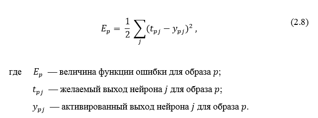
The magnitude of the error is determined by the formula 2.8 root-mean-square error:
The non-activated state of each neuron j for the image p is written as a weighted sum using the formula 2.9:

The output of each neuron j is the value of the activation function.
 which puts the neuron in an activated state. As an activation function, any continuously differentiable monotonic function can be used. The activated state of the neuron is calculated by the formula 2.10:

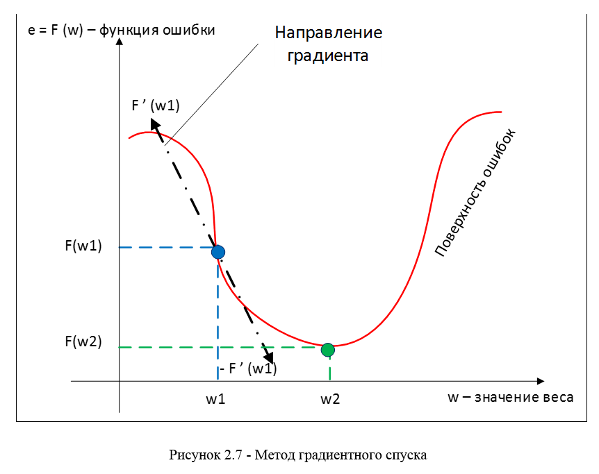
As a method of minimizing the error, the method of gradient descent is used, the essence of this method comes down to finding the minimum (or maximum) of the function due to movement along the gradient vector. To search for a minimum, the movement must be carried out in the direction of the antigradient. Gradient descent method in accordance with Figure 2.7.
The gradient of the loss function is a vector of partial derivatives, calculated by the formula 2.11:

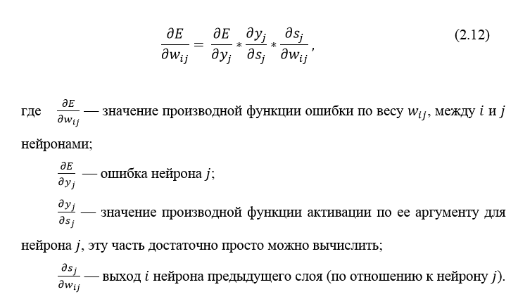
The derivative of the error function for a particular image can be written by the chain rule, formula 2.12:
Neuron error usually written as a symbol δ (delta). For the output layer, the error is defined explicitly, if we take the derivative of formula 2.8, we get t minus y , that is, the difference between the desired and the obtained output. But how to calculate the error for hidden layers? To solve this problem, an algorithm for back propagation of an error was invented. Its essence lies in the sequential calculation of errors of hidden layers using the error values of the output layer, i.e. error values propagate through the network in the opposite direction from the output to the input.
Error δ for the hidden layer is calculated by the formula 2.13:

The error propagation algorithm is reduced to the following stages:
The algorithm for back propagation of an error in a multilayer perceptron is shown below:
Up to this point, the cases of error propagation through the perceptron layers, that is, the output and hidden, have been considered, but in addition to them, there are subsample and convolutional networks in the convolutional neural network.
The calculation of the error on the subsample layer is presented in several variants. The first case, when the subsampling layer is in front of a fully connected one, then it has neurons and connections of the same type as in the fully connected layer, respectively, calculating δ error is no different from calculating δ of the hidden layer. The second case, when the subsampling layer is in front of the convolutional layer, the calculation of δ occurs by reverse convolution. To understand convolution back, you first need to understand ordinary convolution and the fact that the sliding window on the feature map (during direct signal propagation) can be interpreted as a normal hidden layer with connections between neurons, but the main difference is that these connections are shared, that is, one connection with a specific weight value may be in several pairs of neurons, and not just one. Interpretation of the convolution operation in the usual multilayer form in accordance with Figure 2.8.
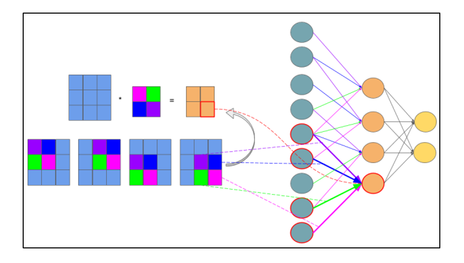
Figure 2.8 - Interpretation of a convolution operation into a multi-layered view, where links with the same color have the same weight. The subsample map is marked in blue, the synaptic nucleus is multicolored, and the resulting convolution is orange.
Now that the convolution operation is presented in its usual multi-layered form, it can be intuitively understood that the deltas are calculated in the same way as in the hidden layer of a fully connected network. Accordingly, having previously calculated deltas of the convolutional layer, one can calculate the deltas of the subsampling, in accordance with Figure 2.9.

Figure 2.9 - Calculation of δ sub-sampling layer due to δ convolutional layer and the core
Reverse convolution is the same method of calculating deltas, only in a slightly tricky way, consisting in rotating the nucleus 180 degrees and sliding the process of scanning a convolutional delta map with modified edge effects. In simple words, we need to take the core of the convolutional map (following the subsampling layer) to rotate it 180 degrees and do the usual convolution using previously calculated convolutional map deltas, but so that the scan window extends beyond the map. The result of the operation of the inverse convolution in accordance with Figure 2.10, the cycle of the passage of the inverse convolution in accordance with Figure 2.11.

Figure 2.10 - The result of the operation of the reverse convolution
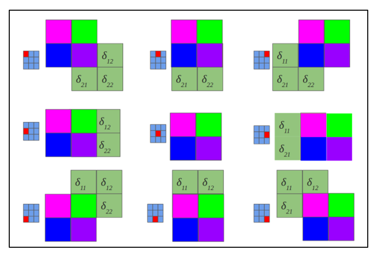
Figure 2.11 - A rotated core 180 degrees scans a convolutional map
Usually the upcoming layer after the convolutional is a subsampling, so our task is to calculate the deltas of the current (convolutional) layer due to the knowledge of the deltas of the subsampling layer. In fact, the delta error is not calculated, but copied. With the direct propagation of the signal, the neurons of the subsampling layer were formed by a non-overlapping scan window on the convolutional layer, during which the neurons with the maximum value were selected.
By presenting the convolution operation in the usual multilayer form (Figure 2.8), one can intuitively understand that the deltas are calculated in the same way as in the hidden layer of a fully connected network.
Error propagation algorithm for convolutional neural network
Reverse error propagation in convolutional layers
one and two
Back propagation of error in perceptron
You can also read the Makarenko's dissertation in the RSL: ALGORITHMS AND PROGRAM CLASSIFICATION SYSTEM
Training convolutional neural network
At the initial stage, the neural network is untrained (unconfigured). In a general sense, learning is the sequential presentation of an image to the input of a neural network, from the training set, then the resulting answer is compared with the desired output, in our case it is 1 - the image represents a person, minus 1 - the image represents a background (not the person), the difference between the expected The answer and the result is the result of the error function (delta error). Then this delta needs to be extended to all connected neurons of the network.
Thus, the training of the neural network is reduced to minimizing the error function by adjusting the weights of the synaptic connections between neurons. The error function is the difference between the received answer and the desired one. For example, a face image was submitted to the input, suppose that the output of the neural network was 0.73, and the desired result is 1 (because the face image), we find that the network error is the difference, that is, 0.27. Then the weights of the output layer of the neurons are adjusted in accordance with the error. For neurons of the output layer, their actual and desired output values are known. Therefore, setting up link weights for such neurons is relatively simple. However, the setting is not so obvious for neurons of the previous layers. For a long time, the algorithm for propagating errors across hidden layers was not known.
Error Propagation Algorithm
For learning the described neural network, the backpropagation algorithm was used. This method of teaching a multilayer neural network is called the generalized delta rule. The method was proposed in 1986 by Rumelhart, McCleland and Williams. This marked a revival of interest in neural networks, which began to fade away in the early 70s. This algorithm is the first and the main practically applicable for training multilayer neural networks.
')
For the output layer, the adjustment of the weights is intuitive, but for the hidden layers there has been no known algorithm for a long time. The weights of the hidden neuron should vary in direct proportion to the error of those neurons with which the neuron is associated. That is why the reverse propagation of these errors through the network allows you to correctly adjust the weights of the connections between all layers. In this case, the magnitude of the error function is reduced and the network is trained.
The basic relations of the back propagation method are obtained with the following notation:
The magnitude of the error is determined by the formula 2.8 root-mean-square error:
The non-activated state of each neuron j for the image p is written as a weighted sum using the formula 2.9:
The output of each neuron j is the value of the activation function.
which puts the neuron in an activated state. As an activation function, any continuously differentiable monotonic function can be used. The activated state of the neuron is calculated by the formula 2.10:As a method of minimizing the error, the method of gradient descent is used, the essence of this method comes down to finding the minimum (or maximum) of the function due to movement along the gradient vector. To search for a minimum, the movement must be carried out in the direction of the antigradient. Gradient descent method in accordance with Figure 2.7.
The gradient of the loss function is a vector of partial derivatives, calculated by the formula 2.11:
The derivative of the error function for a particular image can be written by the chain rule, formula 2.12:
Neuron error
usually written as a symbol δ (delta). For the output layer, the error is defined explicitly, if we take the derivative of formula 2.8, we get t minus y , that is, the difference between the desired and the obtained output. But how to calculate the error for hidden layers? To solve this problem, an algorithm for back propagation of an error was invented. Its essence lies in the sequential calculation of errors of hidden layers using the error values of the output layer, i.e. error values propagate through the network in the opposite direction from the output to the input.Error δ for the hidden layer is calculated by the formula 2.13:
The error propagation algorithm is reduced to the following stages:
- direct signal propagation over the network, calculating the state of neurons;
- calculating the error value δ for the output layer;
- backward propagation: sequentially from the end to the beginning for all hidden layers we calculate δ by the formula 2.13;
- update the weights of the network to the previously calculated error δ.
The algorithm for back propagation of an error in a multilayer perceptron is shown below:
Up to this point, the cases of error propagation through the perceptron layers, that is, the output and hidden, have been considered, but in addition to them, there are subsample and convolutional networks in the convolutional neural network.
Calculation of errors on the subsample layer
The calculation of the error on the subsample layer is presented in several variants. The first case, when the subsampling layer is in front of a fully connected one, then it has neurons and connections of the same type as in the fully connected layer, respectively, calculating δ error is no different from calculating δ of the hidden layer. The second case, when the subsampling layer is in front of the convolutional layer, the calculation of δ occurs by reverse convolution. To understand convolution back, you first need to understand ordinary convolution and the fact that the sliding window on the feature map (during direct signal propagation) can be interpreted as a normal hidden layer with connections between neurons, but the main difference is that these connections are shared, that is, one connection with a specific weight value may be in several pairs of neurons, and not just one. Interpretation of the convolution operation in the usual multilayer form in accordance with Figure 2.8.
Figure 2.8 - Interpretation of a convolution operation into a multi-layered view, where links with the same color have the same weight. The subsample map is marked in blue, the synaptic nucleus is multicolored, and the resulting convolution is orange.
Now that the convolution operation is presented in its usual multi-layered form, it can be intuitively understood that the deltas are calculated in the same way as in the hidden layer of a fully connected network. Accordingly, having previously calculated deltas of the convolutional layer, one can calculate the deltas of the subsampling, in accordance with Figure 2.9.
Figure 2.9 - Calculation of δ sub-sampling layer due to δ convolutional layer and the core
Reverse convolution is the same method of calculating deltas, only in a slightly tricky way, consisting in rotating the nucleus 180 degrees and sliding the process of scanning a convolutional delta map with modified edge effects. In simple words, we need to take the core of the convolutional map (following the subsampling layer) to rotate it 180 degrees and do the usual convolution using previously calculated convolutional map deltas, but so that the scan window extends beyond the map. The result of the operation of the inverse convolution in accordance with Figure 2.10, the cycle of the passage of the inverse convolution in accordance with Figure 2.11.
Figure 2.10 - The result of the operation of the reverse convolution
Figure 2.11 - A rotated core 180 degrees scans a convolutional map
Calculation of the error on the convolutional layer
Usually the upcoming layer after the convolutional is a subsampling, so our task is to calculate the deltas of the current (convolutional) layer due to the knowledge of the deltas of the subsampling layer. In fact, the delta error is not calculated, but copied. With the direct propagation of the signal, the neurons of the subsampling layer were formed by a non-overlapping scan window on the convolutional layer, during which the neurons with the maximum value were selected.
Conclusion
By presenting the convolution operation in the usual multilayer form (Figure 2.8), one can intuitively understand that the deltas are calculated in the same way as in the hidden layer of a fully connected network.
Sources
Error propagation algorithm for convolutional neural network
Reverse error propagation in convolutional layers
one and two
Back propagation of error in perceptron
You can also read the Makarenko's dissertation in the RSL: ALGORITHMS AND PROGRAM CLASSIFICATION SYSTEM
Source: https://habr.com/ru/post/348028/
All Articles