Convolutional neural network, part 1: structure, topology, activation functions and training set

Foreword

These articles ( part 2 ) are part of my research at the university, which sounded like this: “Software system for detecting people in a video stream using a convolutional neural network”. The purpose of the work was to improve the speed characteristics in the process of detecting individuals in a video stream. As a video stream, a smartphone camera was used, a desktop PS (Kotlin language) was written to create and train a convolutional neural network, as well as an Android mobile application (Kotlin language), which used a trained network and “tried” to recognize faces from the camera video stream. The results, I say, turned out so-so, to use an exact copy of the topology I proposed at my own risk (I would not recommend).

Introduction

The best results in the field of face recognition were shown by the Convolutional Neural Network or the convolutional neural network (hereinafter referred to as SNS), which is a logical development of the ideas of such national architecture as the cognitron and the neocognitron. Success is due to the possibility of taking into account the two-dimensional topology of the image, in contrast to the multilayer perceptron.

Convolutional neural networks provide partial resistance to scale changes, offsets, turns, angle changes and other distortions. Convolutional neural networks combine three architectural ideas to ensure invariance to zoom, rotate shear, and spatial distortion:
')

• local receptor fields (provide local two-dimensional neuron connectivity);
• common synaptic coefficients (provide detection of certain features anywhere in the image and reduce the total number of weights);
• hierarchical organization with spatial subsamples.

At the moment, the convolutional neural network and its modifications are considered the best in accuracy and speed algorithms for finding objects on the scene. Beginning in 2012, neural networks occupy the first places in the well-known international competition for image recognition, ImageNet.



That is why in my work I used a convolutional neural network based on the principles of neocognitron and supplemented with training in the back-propagation error algorithm.

The structure of the convolutional neural network

SNA consists of different types of layers: convolutional layers, subsampling (subsampling) subsampling layers and layers of the “ordinary” neural network - the perceptron, in accordance with Figure 1.


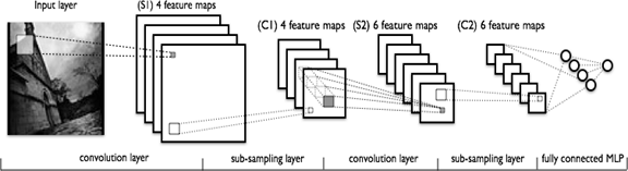
Figure 1 - convolutional neural network topology

The first two types of layers (convolutional, subsampling), alternating with each other, form the input feature vector for a multilayer perceptron.

The convolution network received its name from the operation name — convolution, the essence of which will be described later.

Convolutional networks are a good middle ground between biologically plausible networks and a conventional multilayer perceptron. Today, the best results in image recognition are obtained with their help. On average, the recognition accuracy of such networks exceeds the usual ANNs by 10-15%. SNS is a key technology of deep learning.

The main reason for the success of the SNA was the concept of common weights. Despite their large size, these networks have a small number of adjustable parameters compared to their ancestor, the neocognitron. There are variants of the SNA (Tiled Convolutional Neural Network), similar to the neocognitron, in such networks occurs, a partial rejection of the associated weights, but the learning algorithm remains the same and is based on the back propagation of the error. SNS can quickly work on a sequential machine and quickly learn through pure paralleling of the convolution process on each map, as well as reverse convolution when an error is spread over the network.

The figure below shows the visualization of convolution and subsample:

Convolutional neural network topology

Determining the network topology focuses on the problem being solved, data from scientific articles and its own experimental experience.

The following steps can influence the choice of topology:

• define the task to be solved by a neural network (classification, forecasting, modification);
• define constraints in the problem being solved (speed, accuracy of response);
• define input (type: image, sound, size: 100x100, 30x30, format: RGB, in grayscale) and output data (number of classes).

The task solved by my neural network is the classification of images, specifically individuals. The imposed restrictions on the network is the response speed - no more than 1 second and recognition accuracy of at least 70%. The overall network topology is in accordance with Figure 2.


Figure 2 - The convolutional neural network topology

Input layer

The input data are colored images of type JPEG, size 48x48 pixels. If the size is too large, the computational complexity will increase, respectively, the limitations on the speed of response will be violated, the determination of the size in this problem is solved by the selection method. If you choose a size that is too small, the network will not be able to identify the key features of the faces. Each image is divided into 3 channels: red, blue, green. Thus, 3 images of 48x48 pixels are obtained.

The input layer takes into account the two-dimensional topology of images and consists of several maps (matrices), the map can be one, if the image is represented in shades of gray, otherwise there are 3, where each map corresponds to an image with a specific channel (red, blue and green) .

The input data of each specific pixel value are normalized in the range from 0 to 1, according to the formula:

Convolutional layer

A convolutional layer is a set of maps (another name is feature maps, in everyday life these are ordinary matrices), each map has a synaptic nucleus (in different sources it is called differently: a scanning core or a filter).

The number of cards is determined by the requirements of the task; if you take a large number of cards, the recognition quality will increase, but the computational complexity will increase. Based on the analysis of scientific articles, in most cases it is proposed to take the ratio of one to two, that is, each card of the previous layer (for example, the first convolutional layer, the previous one is the input one) is associated with two maps of the convolutional layer, in accordance with Figure 3. Number of cards - 6


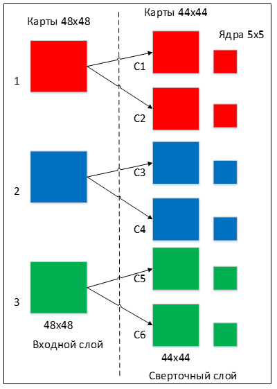
Figure 3 - Organization of links between the maps of the convolutional layer and the previous one

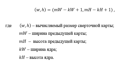
The size of all maps of the convolutional layer is the same and is calculated by the formula 2:



The kernel is a filter or a window that slides over the entire area of ​​the previous map and finds certain attributes of objects. For example, if the network was trained on multiple faces, then one of the nuclei could, in the learning process, produce the largest signal in the eye, mouth, eyebrow or nose, another core could detect other signs. Kernel size is usually taken in the range from 3x3 to 7x7. If the size of the nucleus is small, it will not be able to isolate any signs, if too large, then the number of connections between neurons increases. Also, the core size is chosen so that the size of the maps of the convolutional layer is even, this allows us not to lose information when reducing the dimension in the subsample layer described below.

The nucleus is a system of shared weights or synapses, it is one of the main features of the convolutional neural network. In a conventional multilayer network there are a lot of connections between neurons, that is, synapses, which slows down the detection process very much. In the convolutional network, on the contrary, the total weights reduces the number of connections and allows us to find the same feature throughout the image area.



Initially, the values ​​of each map of the convolutional layer are equal to 0. The values ​​of the weights of the nuclei are set randomly in the range from -0.5 to 0.5. The kernel slides over the previous map and performs a convolution operation, which is often used for image processing, the formula:



Informally, this operation can be described as follows: we pass the window of kernel size g with a given step (usually 1) the entire image f, at each step we elementwise multiply the window contents by the kernel g, the result is summed up and written into the result matrix, as shown in Figure 4.


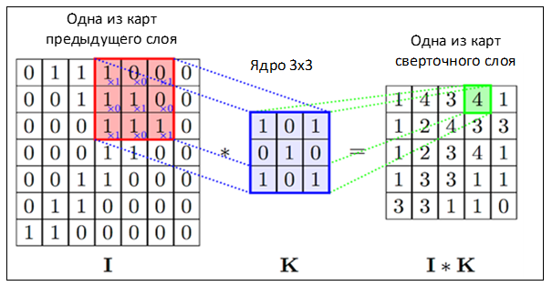
Figure 4 - The operation of convolution and obtaining the values ​​of the convolutional map (valid)


The operation of convolution and obtaining the values ​​of the convolutional map. The core is shifted, the new map is the same size as the previous one (same)

However, depending on the method of processing the edges of the original matrix, the result may be less than the original image (valid), the same size (same) or larger (full), in accordance with Figure 5.


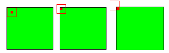
Figure 5 - Three types of convolution of the original matrix

In a simplified form, this layer can be described by the formula:



In this case, due to the edge effects, the size of the original matrices is reduced, the formula:

Sub-election layer

The subselection layer also, like the convolutional one, has maps, but their number coincides with the previous (convolutional) layer, there are 6 of them. The purpose of the layer is to reduce the dimension of the maps of the previous layer. If at the previous convolution operation some signs have already been identified, then such a detailed image is no longer needed for further processing, and it is compacted to less detailed. In addition, filtering already unnecessary parts helps not to retrain.
In the process of scanning by the core of the subsampling layer (filter) of the map of the previous layer, the scanning core does not intersect, unlike the convolutional layer. Usually, each map has a core of 2x2, which allows reducing previous maps of the convolutional layer by 2 times. The entire attribute map is divided into 2x2 cells, from which the maximum values ​​are selected.

Usually, the activation function RelU is used in the subsample layer. The subsample operation (or MaxPooling - the choice of the maximum) in accordance with Figure 6.


Figure 6 - Formation of a new map of the subsample layer based on the previous map of the convolutional layer. Subsample operation (Max Pooling)

Formally, a layer can be described by the formula:

Full bonded layer

The last of the types of layers is the layer of the usual multilayer perceptron. The purpose of the layer is the classification, it models a complex non-linear function, which, while optimizing, improves the quality of recognition.



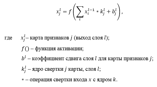
The neurons of each map of the previous subsample layer are associated with one neuron of the hidden layer. Thus, the number of neurons in a hidden layer is equal to the number of maps of a subsampling layer, but connections may not necessarily be such, for example, only a part of the neurons of one of the cards in the subsample layer is associated with the first neuron of the hidden layer, and the rest with the second, or all neurons of the first maps are connected with neurons 1 and 2 of the hidden layer. The calculation of the values ​​of the neuron can be described by the formula:

Output layer

The output layer is connected to all neurons of the previous layer. The number of neurons corresponds to the number of recognizable classes, that is, 2 is a face and not a face. But to reduce the number of connections and calculations for the binary case, you can use a single neuron and using the hyperbolic tangent as an activation function, the output of a neuron with a value of -1 means belonging to the “not a person” class, on the contrary, the output of a neuron with a value of 1 means that it belongs to the class individuals.

Select the activation function

One of the stages of the development of a neural network is the choice of the activation function of neurons. The type of activation function largely determines the functionality of the neural network and the method of training this network. The classical algorithm for back propagation of errors works well on two-layer and three-layer neural networks, but with a further increase in the depth it begins to experience problems. One of the reasons is the so-called attenuation of the gradients. As the error propagates from the output layer to the input layer, each current layer multiplies the current result by the derivative of the activation function. The derivative of the traditional sigmoid activation function is less than unity in the entire domain of definition, therefore, after several layers, the error will become close to zero. If, on the contrary, the activation function has an unlimited derivative (like, for example, a hyperbolic tangent), then an explosive increase in the error as it propagates can occur, which will lead to instability of the learning procedure.

In this paper, the hyperbolic tangent is used as the activation function in the hidden and output layers, and ReLU is used in the convolutional layers. Consider the most common activation functions used in neural networks.

Sigmoid activation function

This function belongs to the class of continuous functions and takes an arbitrary real number at the input, and at the output it gives a real number in the range from 0 to 1. In particular, large (modulo) negative numbers turn into zero, and large positive ones turn into one. Historically, sigmoid has been widely used since its output is well interpreted as the level of neuron activation: from no activation (0) to fully saturated activation (1). Sigmoid (sigmoid) is expressed by the formula:



Graph of sigmoidal function in accordance with the figure below:



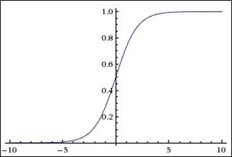
The extremely undesirable property of sigmoids is that when the function is saturated from one side or another (0 or 1), the gradient in these areas becomes close to zero.

Recall that in the process of back propagation of an error, the given (local) gradient is multiplied by the total gradient. Therefore, if the local gradient is very small, it actually nulls the overall gradient. As a result, the signal will almost not pass through the neuron to its weights and recursively to its data. In addition, you should be very careful when initializing the weights of sigmoid neurons to prevent saturation. For example, if the initial weights are too large, most neurons will become saturated, with the result that the network will be poorly trained.

Sigmoidal function is:

• continuous;
• monotonically increasing;
• differentiable.

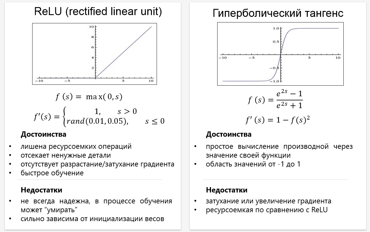
Activation function hyperbolic tangent

In this paper, the hyperbolic tangent is used as the activation function for the hidden and output layers. This is due to the following reasons:

• symmetric activation functions such as hyperbolic tangent provide faster convergence than the standard logistic function;
• the function has a continuous first derivative;
• a function has a simple derivative that can be calculated through its value, which saves computation.

The graph of the function of the hyperbolic tangent is shown in the figure:

Activation function ReLU

It is known that neural networks are capable of approximating an arbitrarily complex function if there are enough layers in them and the activation function is nonlinear. Activation functions like sigmoid or tangential are non-linear, but lead to problems with fading or increasing gradients. However, you can use a much simpler option - rectified linear activation function (rectified linear unit, ReLU), which is expressed by the formula:



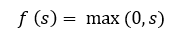
Graph of the ReLU function in accordance with the figure below:



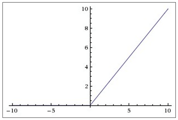
Benefits of using ReLU:

• its derivative is equal to either one or zero, and therefore the growth or decay of gradients cannot occur, since multiplying the unit by the delta error, we get the delta error, if we would use another function, for example, the hyperbolic tangent, then the delta error could either decrease or increase, or remain the same, that is, the derivative of the hyperbolic tangent returns a number with a different sign and the magnitude that can greatly affect the attenuation or growth of the gradient. Moreover, the use of this function leads to the thinning of the scales;
• calculating sigmoids and hyperbolic tangent requires resource-intensive operations, such as exponentiation, while ReLU can be implemented using a simple threshold transformation of the activation matrix at zero;
• cuts off unnecessary parts in the channel with a negative output.

Among the shortcomings, it can be noted that the ReLU is not always sufficiently reliable and in the learning process can fail (“die”). For example, a large gradient passing through a ReLU can lead to such an update of the balance that the neuron is never activated again. If this happens, then, from now on, the gradient passing through this neuron will always be zero. Accordingly, this neuron will be irreversibly disabled. For example, if the learning rate is too high, it may turn out that up to 40% of the ReLUs are “dead” (that is, never activated). This problem is solved by choosing the appropriate learning speed.

Training samples used in experiments

A training set consists of positive and negative examples. In this case, from individuals and “non-individuals”. The ratio of positive to negative examples 4 to 1, 8000 positive and 2000 negative.

The LFW3D database [7] was used as a positive training sample. It contains color images of frontal faces such as JPEG, size 90x90 pixels, in the amount of 13000. The database is provided via FTP, access is carried out with a password. To receive a password, you must fill out a simple form on the main page of the site, where you can enter your name and email. An example of people from the database is shown in accordance with the figure below:



As a negative teaching examples used database SUN397 [8], it contains a huge number of various scenes, which are divided into categories. A total of 130,000 images, 908 scenes, 313,000 scene objects. The total weight of this base is 37 GB. The categories of images are quite different and allow you to choose a more specific environment where the final PS will be used. For example, if it is known a priori that the face detector is intended only for indoor recognition, then there is no point in using a training sample of nature, sky, mountains, etc. For this reason, the author selected the following categories of images: living room, study, classroom, computer room. Examples of images from the SUN397 training set are shown in accordance with the figure below:

results

Direct propagation of a signal from an input image of 90x90 pixels takes 20 ms (on a PC), 3000 ms in a mobile application. When detecting a face in a video stream at a resolution of 640x480 pixels, it is possible to detect 50 non-overlapping areas with a size of 90x90 pixels. The results obtained with the selected network topology are worse than the Viola-Jones algorithm.

findings

Convolutional neural networks provide partial resistance to scale changes, offsets, turns, angle changes and other distortions.

The core is a filter that slides over the entire image and finds signs of a face in any place (invariance to displacements).

The sub-sample layer gives:

• an increase in the speed of calculations (at least 2 times), due to a decrease in the dimension of the maps of the previous layer;
• filtering already unnecessary parts;
• search for higher level traits (for the next convolutional layer).

The last layers are the layers of the usual multilayer perceptron. Two fully connected and one day off. This layer is responsible for the classification, from a mathematical point of view, models a complex non-linear function, optimizing which improves the quality of recognition. The number of neurons in layer 6 by the number of maps of signs of a subsample layer.

Possible improvements

• consider neural networks Fast-RCNN, YOLO;
• parallelization of the learning process on graphics processors;
• use Android NDK (C ++) to improve performance

Training convolutional neural network is described in the second part .

Links

- What is a convolutional neural network

- Learning sets:
Effective Face Frontalization in Unconstrained Images // Effective Face.
SUN Database // MIT Computer Science and Artificial Intelligence Laboratory

- Information on convolutional neural networks

- About neural network learning functions

- Types of neural networks (similar neural network classification scheme)

- Neural networks for beginners: one and two .