Optimization of multi-stage compressors for energy consumption for adiabatic gas compression

Introduction

In 1934, the Swiss firm Brown-Boveri, based on theoretical work, Stodoly first created a multi-stage axial compressor with an efficiency of 84%. Soon, axial compressors began to be used successfully by this company for gas turbine installations.

Multistage axial compressors [1]

A schematic diagram of an axial multistage compressor is shown in the figure:
')


The axial multi-stage compressor consists of a series of sequentially arranged guide vanes 6 fixed in the housing 7 and working blades 5 located on the drum rotor 11. As compression progresses, the volume of air decreases and, consequently, the heights of the blades decrease.

Rotating, the rotor blades communicate kinetic energy to the gas. When moving along the expanding channels of the working blades, the relative velocity of the air decreases, the kinetic energy of the flow decreases with a corresponding increase in pressure in it.

The change in the relative flow rate in the channel of the working blades is associated with the consumption of energy supplied to the compressor.

In the expanding channels of the guide vanes there is a further increase in air pressure and a decrease in its speed. In the flow part of the compressor air enters through the inlet pipe 1 and the guide unit 4, from where, after passing the channels of the working vanes 5 and guide vanes 6, it enters the straightening apparatus 8.

The guide device provides the necessary direction to the air flow before entering the first stage, and the rectifying device provides axial exit to the diffuser 9 and further to the outlet 10.

The number of stages of compression in this design is determined by the number of blades 5, located on the drum rotor 11.

Multistage piston compressors [2]

To obtain a compressed gas of higher pressure (0.1–2 MPa and above), multistage compressors with intermediate gas cooling are used after each stage.

The essence of multi-stage compression can be explained by the example of a two-stage compressor, whose diagram and ideal (with Vo = 0) indicator diagram is shown in the figure:



In the first stage 1, the gas is compressed by polytrope 1–2 to the pressure P2, and then it enters the intermediate cooler 3, where it is cooled to the initial temperature T1. The hydraulic resistance of the refrigerator along the air path is made small. This suggests that the cooling process is 2–3 isobaric.

After the refrigerator, the gas enters the second stage 2, where it is compressed along polytrope 3–4 to pressure P3. If compression to the pressure P3 were carried out in an ideal single-stage compressor (line 1–2 '), then the value spent per cycle of operation would be determined by the area of ​​012'b0.

With a two-stage compression with intermediate cooling, this work is numerically equal to the area 01234b0. The shaded area corresponds to the saving of work per cycle under two-stage compression.

Multistage gas compression [3]

When multi-stage isentropic compression of gas from the initial pressure Po to the final pressure Pn , it is desirable to establish such intermediate pressures at which the total energy expended in compression would be minimal.

The gas is cooled isobaric to its initial temperature T, after each adiabatic compression. The energy expenditure at the n-stage is determined from the equation:



where: m is the number of kmols of compressible gas; R is the universal gas constant, ;
T is the initial gas temperature, K; γ is the ratio of the specific heats of gas at constant pressure and constant volume, in the work it is assumed γ = 1.4; xn is the gas pressure after compression in the n stage.

Formulation of the problem

1. Find the pressure distribution at the output of the adiabatic compression stages at which the energy spent on compression 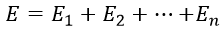will be minimal;

2. Determine the effect of the number of degrees of compression on the minimum energy of compression at the same values ​​of the initial and final pressures.

Solution of the problem by means of the scipy library. optimize

First, we consider five compression levels in accordance with the design diagram shown in the figure:




We get:
Optimizer operation time: 0.0



Increase the number of compression steps by one according to the following listing:


We get:
Optimizer work time: 0.005



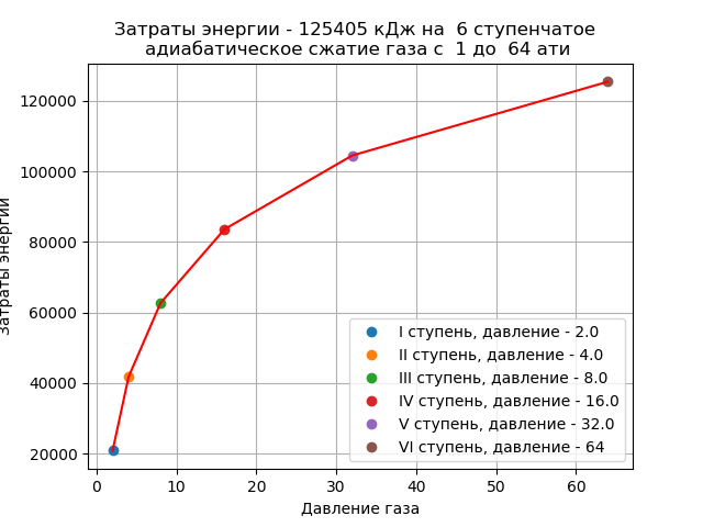
Comparing the given graphs, it is possible to determine the reduction of energy consumption for adiabatic compression of gas:

(149024 -125405) * 100/149024 = 15, 85%

Conclusion: an increase in the number of compression steps by only one unit saves almost 16% of the energy spent on the adiabatic compression of gas in a multi-stage compressor.

However, this is only one type of energy expended. It is clear that the introduction of an additional step will lead not only to additional costs in the manufacture, but also to additional operating costs, due to an increase in engine power and cooling system section.

The optimal option should be chosen taking into account all types of costs, but this is a completely different task.

Findings:

1. Found the pressure distribution at the output of the adiabatic compression stages at which the energy spent on adiabatic compression is minimal;

2. Increasing the number of compression stages by only one unit saves almost 16% of the energy spent on adiabatic gas compression in a multi-stage compressor.

References:

1. Compressors of gas turbine units (GTU).
2. Multistage compressor.
3. Fan - Lien - Cen, Wang, Chu - Sen. The discrete maximum principle. - M, "Peace", 1967.-176 p.