Python for teaching science informatics: Simulating Queuing Systems

annotation

In this article, we present a methodology for the initial development of scientific informatics, based on modeling in training. We offer multiphase queuing systems as a basis for the objects under study. We use Python and parallel computing to implement models, with the provision of software code and the results of stochastic modeling.

1. Introduction and Prehistory

In our study, we understand the meaning of the term “scientific computer science” as the use of computers for analyzing and solving scientific and engineering problems. We distinguish them from simple numerical calculations. The use of scientific informatics in teaching is always a difficult task, both for the student and for the teacher. This learning process deals with many technical and interdisciplinary issues, and also requires the synchronization of mathematical knowledge with computer science. To overcome these difficulties, we offer a set of teaching principles and a methodology that is based on a constructivist approach to learning and provides an appropriate structural basis for the teacher. All this allows students to conduct a series of computational experiments with computer models. This approach is associated with the knowledge of mathematics and programming, which, in turn, are taught in the course of the main training course and are closely related to it. We will consider the section of computational statistics as an introductory section of scientific informatics and as a possible field of application of this study. Below is the background of this methodology.

1.1. Science Informatics

Karniadax and Kirby II defined “computer informatics as` hearts' of imitational research ”. The authors propose a “holistic approach of numerical algorithms, modern programming methods and parallel computing ... Often such concepts and similar tools are periodically studied in various, related topics, courses and textbooks, and the relationship between them becomes immediately apparent. The need to integrate concepts and tools usually becomes apparent after completing the course, for example, during the first post-graduate work or when writing theses for a thesis, thus forcing the student to synthesize an understanding of three independent areas into one to obtain the required solution. Although this process is undoubtedly very valuable, it takes a lot of time and, in many cases, it may not provide an effective combination of concepts and tools. From a pedagogical point of view, to enhance the understanding of scientific informatics topics, a holistic integrated approach can stimulate the student to several disciplines at once. Figure 1 presents the definition of scientific computer science as the intersection of numerical mathematics, computer science and modeling [16].

Fig. 1. Scientific informatics.

1.2. Constructivism in learning

Kane and Kane in their basic research [6] proposed the basic principles of constructivism in teaching. One of the most important for us is the following: "The brain processes the parts and the whole simultaneously."
')
Thus, a well-organized learning process demonstrates the underlying details and ideas. Using the approach based on modeling, after the creation of a simulation model, the objectives of the study become apparent. This allows us to observe the results and form the appropriate conclusions.

1.3. Simulation-based learning: why models?

Gibbons introduces a simulation-based training program in 2001 [9]. Highlighting the following fundamental principles:

• The learner gains experience by interacting with models;
• The student solves scientific and engineering problems by experimenting with the model;
• Consideration and formulation of problems;
• Defining specific learning objectives;
• Presentation of all necessary information in the context of the decision.

Millard et al. [30] offer a lightweight learning model using “interactive simulation”. The authors present modern computer technologies based on a “promising methodology” based on “system dynamics”. “Practical experience includes designing interactive ... models, as well as their use for testing hypotheses and experiments.”

Lerer and Schauble [25] focus on experiments with different representations of the model: “Student learning is enhanced when the student has the ability to create and revise several versions of models, and then compare the adequacy of the description of these different models.”

1.4. Scientific informatics at the basis of education: experiments with models

Xue [40] proposes “teaching reform in teaching based on“ scientific informatics ”through modeling and imitations.” He advises “... to use modeling and imitation to solve actual problems of programming, modeling and data analysis ...”. Simulation based training is used in math education. Many models are built using the software "Geogebra" [33]. Models play a major role in scientific education [7,18].

1.5. Stochastic simulation of queuing systems

We propose the use of queuing systems due to the simplicity of their initial definitions and due to the wide possibilities of modeling and imitations. The theory of Mass Service is well known and the modeling of Mass Service Systems (CMS) is widely used in science [4,19] and education [13,36]. Multiphase queuing systems are a good platform for student experimentation, as is the use of parallel computing. There are also a number of interesting theoretical results for the study and study [12].

1.6. Python in science based computer science education

Python is one of the most popular programming languages ​​for scientists and educators [21–23]. Python is widely used in industrial scientific computing [14]. Langtangen reports on the long-term experience of using Python as the primary language for teaching Informatics at the University of Oslo [24]. Python is advancing as the first language for learning programming [38], as well as for in-depth study of computational methods [3,20,34].

2. Basics

Before embarking on modeling, we will define key approaches that we will use in the process. In this chapter we will touch on the generation of random numbers and probability distributions, stochastic modeling. Consider the elementary probability theory. The main task of these experiments will be experimental proof of the Central Limit Theorem. Models and experiments with these models clarify the principle of pseudo- and quasi-random number generators, as well as an understanding of the exponential distribution. This can provide a basis for more detailed experiments with QS models.

2.1. Random Variables and Distributions

All elements of the theory of probability are traditionally considered difficult to understand and are always in the sphere of interests of international educational institutions [15]. At the same time, these questions occupy an important role in scientific research [10]. A modeling approach makes it easier to understand this material. The model, which we consider in this article, is a simple model of throwing one or several dice, starting with one and ending with several.

The task of these introductory experiments is quite complex. We will not only consider probability distributions, but also touch on modeling and parallel computing. We will also take one step forward in scientific research: we experimentally prove the Central Limit Theorem.

We will start by generating random numbers (without affecting the distribution). Then we explain the uniformly distributed random variables. Discussions about true chance and quasi chance are presented by the authors [26, 35]. For advanced students, a series of experiments with a Python pseudo-random variable generator will be presented. At the initial stage, for clarity of study, we will increase the number of tests, observing the result of modeling. At the next stage, we will move on to more complex experiments and parallel computations. We will use the Python random variable module for simulation, and the mpi4py library for parallel computing. The Python random variable module is based on a pseudo-random number generator for various distributions. For example: random.randint (a, b) returns a random integer N, where a ≤ N ≤ b and random.expovariate (lambd) returns exponentially distributed random variables with the parameter 'lambd'. For more information, refer to the Python documentation. The programming of the cube tossing model is shown in Fig.2.

import pylab import random number_of_trials =100 ## Here we simulate the repeated throwing of a single six-sided die list_of_values = [] for i in range(number_of_trials): list_of_values.append(random.randint( 1,6)) print "Trials =", number_of_trials, "times." print "Mean =", pylab.mean(list_of_values) print "Standard deviation =", pylab.std(list_of_values) pylab.hist(list_of_values, bins=[0.5,1.5,2.5,3-5,4.5,5.5,6.5]) pylab.xlabel('Value') pylab.ylabel('Number of times') pylab.show() 

Fig. 2. Programming the model of throwing one cube in Python

The simulation results of throwing one die are presented in Figure 3.


Fig. 3. Simulation results of one die toss

Next, consider the case of tossing two playing dice. The main idea at this stage is to explain the CLT using an experiment with a different number of cubes. Figure 4 demonstrates this idea.


Fig. 4. Comparison of probability density functions

The learning process continues by modifying the code to simulate throwing two cubes in such a way as to begin to consider the case with several cubes. The code is similar to the code with one die, except for the two lines of code below:

 ... list_of_values.append(random.randint(1, 6) + random.randint(1, 6)) ... pylab.hist(list_of_values, pylab.arange(1.5, 13.5, 1.0)) ... 

The result of the calculations in the case of two cubes is presented in Figure 5.


Fig. 5. The case of two dice

Now we can consider the normal distribution. The task, at this stage, is to show how the previous case with several cubes correlates with the normal distribution. The next task will introduce us to the average value and standard deviation. The code remains the same as in the case of a single die, with the exception of the instructions below:

 ... list_of_values.append(random.normalvariate(7, 2.4)) ... 

The simulation results for the normal distribution are presented in Figure 6.


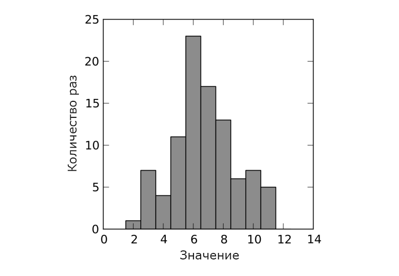
Fig. 6. Simulation result for normal distribution

The final step is to demonstrate the exponential distribution. The exponential distribution is used to simulate the distribution (duration) of the intervals between the arrival times of requirements in different types of systems. The results of their modeling are presented in Figure 7 and 8.

 import pylab import random number_of_trials = 1000 number_of_customer_per_hour = 10 ## Here we simulate the interarrival time of the customers list_of_values = [] for i in range(number of trials): list_of_values.append(random.expovariate(number_of_customer_per_hour)) mean=pylab.mean(list_of_values) std=pylab.std(list_of_values) print "Trials =", number_of_trials, "times" print "Mean =", mean print "Standard deviation =", std pylab.hist(list_of_values,20) pylab.xlabel('Value') pylab.ylabel('Number of times') pylab.show() 

Fig. 7. Python Model for Exponential Distribution


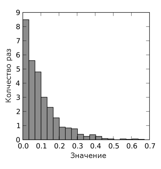
Fig. 8. Simulation result for exponential distribution

2.2. Stochastic simulation

Stochastic modeling is an important element of scientific informatics. We will focus on the Monte Carlo method [10,11,27]. After the model has been built, we can generate random variables and experiment with various system parameters. In this article, the key point of Monte Carlo experiments is to repeat the test many times in order to accumulate and integrate the results. The simplest application was described in the previous section. Increasing the number of tests, we will increase the accuracy of the simulation results.

Here the student must conduct a certain number of experiments using this simple model by increasing the number of tests. By increasing the number of cubes and the number of tests, the student will face a relatively long calculation time. This is a great reason to use parallel computing. The Python model for several playing cubes is presented in Figure 9. And the simulation results are presented in Figure 10. The next step will be to consider more general issues related to various queuing systems. A brief introduction to the QS classification is presented in the next part of this article. We begin the study with the M / M / 1 system and more complex queuing systems. The basic concepts of stochastic processes will be covered in detail in this part of the article. As a possible example, we can offer the problem of studying the output stream. We prove that the output of the M / M / 1 system is a Poisson flow. Thus, the collected data will be presented in the form of a built output empirical histogram.

 import pylab import random number_of_trials = 150000 number_of_dice = 200 ## Here we simulate the repeated throwing ## of a number of single six-sided dice list_of_values = [] for i in range(number_of_trials): sum=0 for j in range(number_of_dice): sum+=random.randint(1,6) list_of_values.append(sum) mean=pylab.mean(list_of_values) std=pylab.std(list_of_values) print "Trials =", number_of_trials, "times" print "Mean =", mean print "Standard deviation =", std pylab.hist(list_of_values,20) pylab.xlabel('Value') pylab.ylabel('Number of times') pylab.show() 

Fig. 9. Python simulation model for extended normal distribution


Fig. 10. Simulation result for extended normal distribution

3. Multiphase queuing systems and stochastic modeling

Below is an introductory description of the QS, taking into account the nuances of modeling and stochastics.

3.1. Mass Service Systems

A simple queuing system consists of one serving device that processes incoming requests. The general scheme of a simple queuing system is presented in Fig. 11. In general, a QS consists of one or several servicing devices that process incoming requests. A variant of one or several stages of service with one or several servicing devices in each phase is also possible. Arriving clients who find all servers busy are joining one or more queues before serving devices. There are many applications that can be used to model QS, such as production systems, communication systems, maintenance systems and others. General QS can be characterized by three main components: the flow of applications, the maintenance process and the method of servicing the queue. Entries can come from several limited or unlimited sources.


Fig. 11. Simple SMO.

The application process describes how applications come into the system. Define
$$$\ alpha_i$ as the time interval between the arrival of applications between $$$(i -1)$ and $$$i$ application, expected (average) time between receipt of applications as $$$E (\ alpha)$ and frequency of bids as $$$\ lambda = \ frac {1} {E (\ alpha)}$

Also define $$$s$ as the number of servicing devices. The maintenance mechanism is determined by this number. Each service device has its own queue, as well as a probabilistic distribution of application service time.

Define $$$s_i$ how time is service $$$i$ th application, $$$E (s)$ as the average service time of the application and $$$\ mu = \ frac {1} {E (s)}$ as the speed of service applications.

The rule that the server uses to select the next application from the queue is called the QS queue discipline. The most frequent disciplines of the queue: Priority - customers are served in order of importance. FIFO - first come first served; LIFO - stack, the last one came first served. Extended Kendall systems classification uses 6 characters: A / B / s / q / c / p, where A is the distribution of intervals between incoming requests, B is the distribution of service intervals, s is the number of servers, q is service disciplines (omitted for FIFO) , c - system capacity (omitted for infinite queues), p - number of possible requests (omitted for open systems) [17.37]. For example, M / M / 1 describes the Poisson flow at the input, one exponential service device, one infinite FIFO queue, and an infinite number of requests.

SMOs are used to model and study various areas of science and technology. For example: we can model and study production or transport systems using queuing theory. Moreover, service requests are considered as requests, and maintenance procedures as a maintenance mechanism. The following example is: computers (terminal requests and server responses, respectively), computer multidisk memory systems (data write / read requests, shared disk controller), trunked radio communication (telephone signals, repeaters), computer networks (queries, channels) [39 ]. In biology, queuing theory can be used to model enzyme systems (proteins, general enzymes). In biochemistry, a queuing network model can be used to study the regulatory chain of the lac operon.

3.2. Why multiphase?

Consider a multiphase QS, which consists of several servicing devices that are connected in series and have an unlimited number of applications. The time between bids and processing times are independent and exponentially distributed. The queue is endless with FIFO service discipline. Multiphase QS naturally reflects the topology of multi-core computer systems. As we will see later, each model can be easily written in a programming language, studied and modified. The model also allows for a comparative study of various multiprocessing approaches. The multiphase QS model is presented in Figure 12.


Fig. 12. Multiphase QS.

3.3. Theoretical basis

In the case of statistical modeling, we are always faced with the problem of verifying computer code. The question of errors in our program or algorithm is always open. The model is not completely analytical and each time starting the program we have different data on the input / output. Thus, to verify the correctness of the code or algorithm, different approaches are needed (from the one we use in the case of fully deterministic input data). To address this issue, we must apply the theoretical results of some research that can be found in the scientific literature. These results give us a basis for verifying and analyzing the output data, as well as for solving the problem of the correctness of the simulation results [31,32].

We will investigate the time of the application in a multiphase QS. Denote $$$T_j, _n$ as the residence time of the application in the system, $$$S_n ^ {(j)}$ as the service time n- th application of the j -th phase. Will consider $$$\ alpha_k$ as $$$E (\ alpha)$ for the k -th phase.

There is such a constant $$$\ gamma> 0$ such that

$$

$$$ sup_ {n \ geq2} E | S_n ^ {(j)} | ^ {4+ \ gamma} <\ infty, j = 0, 1, 2, ..., k \; (1) \\ \ alpha_k> a_ {k-1}> ...> \ alpha_1> 0 \; (2)$$

Theorem. If conditions (1) and (2) are met, then

$$

$$P \ bigg (\ overline \ lim_ {n \ to \ infty} \ frac {T_ {j, n} - \ alpha_j \ cdot n} {\ widetilde {\ sigma} \ cdot \ alpha (n)} = 1 \ bigg) = \\ P \ bigg (\ underline \ lim_ {n \ to \ infty} \ frac {T_ {j, n} - \ alpha_j \ cdot n} {\ widetilde {\ sigma} \ cdot \ alpha (n) } = -1 \ bigg) = 1, \\ j = 1, 2, ..., 3, k \; ; \ alpha (n) = \ sqrt (2n \ ln \ ln n)$$

3.4. Statistical modeling

After the model is built, we could conduct a series of experiments with this model. This will allow to study some characteristics of the system. We can emit random variables with the expected mean value and calculate (using the recursion equation presented below) the desired values ​​for the study. These values ​​will also be random (we have the stochasticity of the input data of our model - the random time between the arrival of applications and the random service time). As a result, we can calculate some parameters of these random variables (variables): the average value and the probability distribution. We call this method statistical modeling because of the randomness presented in the model. If more accurate results are needed, we must repeat the experiments with our model and then integrate the results, then calculate the integral characteristics: the mean value or standard deviation. This is called the Monte Carlo method and it was described in the article a little higher.

3.5. Recurrence equation

To develop a simulation algorithm previously described by the QS, you need to disassemble some mathematical constructions. The main task is to study and calculate the residence time of the application with the number n in a multi-phase QS consisting of $$$k$ phases. We can give the following recurrence equation [12], we denote: $$$t_n$ - Arrival time $$$n$ th application; $$$S_n ^ {(j)}$ how service time $$$n$ th application $$$j$ -th phase; $$$\ alpha_n = t_n - t_ {n-1}; j = 1, 2, ..., k; n = 1, 2, ..., N.$ . The following recurrence equation holds for the waiting time. $$$T_ {j, n}$ for $$$n$ th application $$$j$ th phase:

$$

$$T_ {j, n} = T_ {j-1, n} + S ^ {j} _n + \ max (T_ {j, n-1} - T_ {j-1, n} - \ alpha_n, 0) ; \\ j = 1, 2, ..., k; n = 1, 2, ..., N; \\ \\ T_ {j, 0} = 0, \ forall j; T_ {0, n} = 0, \ forall n;$$

Assumption. Recurrent equation for calculating the residence time of the application in a multiphase QS.

Evidence. It is true that if time $$$\ alpha_n + T_ {j-1, n} ≥ T_ {j, n-1}$ then waiting time in $$$j$ th phase $$$n$ th application is 0. In this case $$$\ alpha_n + T_ {j-1, n} <T_ {j, n-1}$ waiting time in $$$j$ th phase $$$n$ th application $$$\ omega_j ^ n = T_ {j, n-1} - T_ {j-1, n} - \ alpha_n$ and $$$T_ {j, n} = T_ {j-1, n} - \ omega_j ^ n + S_n ^ {(j)}$ . Taking into account the two cases mentioned above, we end up with an expected result.

Now we can start implementing the necessary algorithms based on all the theoretical results obtained.

4. Python for multiprocessing

Python as a programming language is very popular among scientists and educators and can be very attractive for solving science-oriented problems [3]. Python provides a powerful platform for modeling and simulation, including graphical utilities, a wide variety of mathematical and statistical packages, as well as multiprocessing packages. To reduce execution time, it is necessary to combine Python and C code. All this gives us a powerful modeling platform for generating statistical data and processing results. Key concepts in Python that are also important in modeling are decorators, coroutines, yield expressions, multiprocessing, and queues. These moments are very well considered by Beasley in his book [2]. In spite of this, there are several ways to organize interprocess communication, and we will start with the use of queues, because this is very natural in the light of the study of QS.

Below is a simple example of the advantages of using multiprocessing to increase the efficiency and effectiveness of program code. A student can improve simulation results by using parallel computing on supercomputers or cluster systems [28, 29]. On the one hand, multiprocessing will allow us to compare the multiphase model with multi-core processor resources, and on the other hand, we can use multiprocessing to perform a series of parallel Monte-Carlo tests. We will look at these two approaches in the next section. For motivated students, a brief introduction to multiprocessor processing using Python will be presented next.

We will start by using the mpi4py module. This is important to present the main idea of ​​how MPI works. It simply copies the supplied program to one of the processor cores defined by the user, and integrates the results after using the gather () method. An example of Python code (Fig. 13) and simulation results (Fig. 14) are presented below.

 #!/usr/bin/python import pylab import random import numpy as np from mpi4py import MPI dice=200 trials= 150000 rank = MPI.COMM_WORLD.Get_rank() size = MPI.COMM WORLD.Get_size() name = MPI.Get_processor_name() random.seed(rank) ## Each process - one throwing of a number of six-sided dice values= np.zeros(trials) for i in range(trials): sum=0 for j in range(dice): sum+=random.randint(l,6) values[i]=sum data=np.array(MPI.COMM_WORLD.gather(values, root=0)) if rank == 0: data=data.flatten() mean=pylab.mean(data) std=pylab.std(data) print "Number of trials =", size*trials, "times." print "Mean =", mean print "Standard deviation =", std pylab.hist(data,20) pylab.xlabel('Value') pylab.ylabel('Number of times') pylab.savefig('multi_dice_mpi.png') 

Fig. 13. Python model for extended normal distribution using MPI.


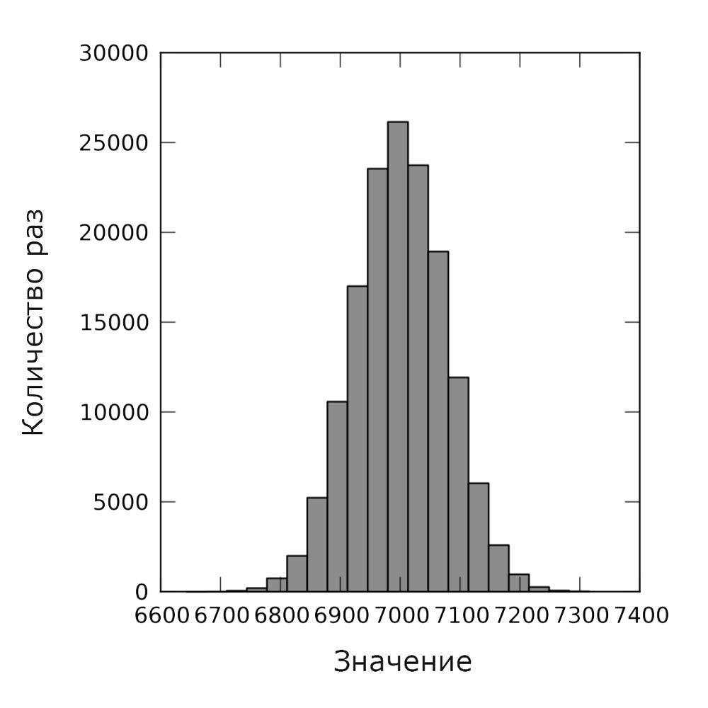
Fig. 14. Normal distribution using MPI.

5. Educational approach based on modeling.

Multiphase QS give us the core to develop an appropriate approach based on modeling. This approach includes the basic concepts described in the previous sections, as well as more complex theoretical results and methods. The main ideas are stochastic in nature: random variables, random number distributions, random number generators, Central Limit Theorem; Python programming constructs:
decorators, coroutines and yeild expressions. More complex results include the following theoretical concepts: the residence time of an application in the system, the recurrent equation for calculating the residence time of an application in the QS, methods of stochastic modeling, and multiprocessor technologies. Figure 15 shows the main scheme describing the educational background.


Fig. 15. Educational approach based on modeling.

All these theoretical and software structures allow the student to conduct an experiment with various models of multiphase QS. The purpose of such experiments is twofold. First, it gives students to understand the following sequence, which is important in any research: theoretical facts necessary for studying, mathematical models, software constructions, computer models, stochastic models, and observation of simulation results. This will give the student a complete picture of general research (Figure 16).


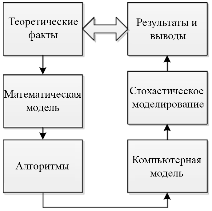
Fig. 16. Field of research

This approach will allow a deeper understanding of stochastic modeling and basic software constructs, such as multiprocessing and parallel programming. These provisions are of paramount importance in the field of scientific computing.

5.1. Experiments with models

In this section, we consider three computer models of multiphase QS. All these models are different in their philosophical and key features. Despite the fact that the purpose of experiments is to create a statistical model and study the main parameters of multiphase systems, the conceptual ideas of these models are completely different. Comparing these basic ideas will help the student understand the fundamental principles that underlie parallel computing, multiprocessing statistical, and simulation modeling.

The first model presented by us is based on real-time recording and we call it a simulation model. It uses the Python multiprocessor module. The accuracy of this model depends on the accuracy and resolution of the time () method. It can be quite low in the case of various general-purpose operating systems, and rather high in the case of real-time systems. The student can change this model using the previously proposed recurrent equation (to calculate the time the application is in the system) and compare the results in both cases.

The following model calculates the residence time of the application in the system and is based on stochastic modeling. The model does not use multiprocessing directly. Multiprocessing is emulated by using yield Python expressions.

The latest model is presented here using the Python MPI mpi4py module. Here the real MPI (multiprocessor) approach is used for statistical modeling and we can, due to this, the number of tests in the Monte Carlo method increases.

In general, the student’s task is to create a series of experiments with the models provided and obtain experimental evidence of the law of the iterated logarithm for the residence time of the application in a multiphase QS.

5.2. Simulation model using multiprocessor service

Below is a simulation model. The main question to study is the difference between the simulation model and the statistical model. Another important issue is the correctness and accuracy of the simulation model. Also important is the question of the accuracy and accuracy of the presented model. The student can study and compare the simulation results, depending on various parameters, such as the interval and frequency of processing, the number of applications and the number of service nodes. The general scheme of the model is shown in Figure 17.


Fig. 17. Simulation model

Program code code consists of two main parts. The first one is intended directly for calculations, and the next one is for building results. The module for calculating contains three main functions: producer () - for receiving applications and placing them first; server () - for service requests; consumer () - to get results. This software model is based on a real simulation and does not use mathematical expressions for calculations. Its accuracy depends on the accuracy of the Python time module and, as a rule, depends on the operating system. Calculation of the work of servicing devices are distributed between different processes within a multiprocessor system. The computer code for the implementation of the above model is presented in Figure 18.

 import multiprocessing import time import random import numpy as np def server(input_q,next_q,i): while True: item = input_q.get() if i==0:item.st=time.time() ## start recording time ## (first phase) timc.sleep(random.expovariate(glambda|i])) ##stop recording time (last phase) if i==M-1 :item.st=time.time()-item.st next_q.put(item) input_q.task_done() print("Server%d stop" % i) ##will be never printed why? def producer(sequence,output_q): for item in sequence: time.sleep(random.expovariate(glambda[0])) output_q.put(ilem) def consumer(input_q): "Finalizing procedures" ## start recording processing time ptime=time.time() in_seq=[] while True: item = input_q.get() in_scq+=[item] input_q.task_done() if item.cid == N-1: break print_results(in_seq) print("END") print("Processing time sec. %d" %(time.time()-ptime)) ## stop recording processing time printf("CPU used %d" %(multiprocessing.cpu_count())) def print_resulls(in_seq): "Output rezults" f=open("out.txt","w") f.write("%d\n" % N) for l in range(M): f.write("%d%s" % (glambda[t],",")) f.write("%d\n" % glambda[M]) for t in range(N-1): f.write("%f%s" % (in_seq[t].st,",")) f.write("%f\n" % (in_seq[N-1].st)) f.close() class Client(object): "Class client" def __init__(self,cid,st): self.cid=cid ## customer id self.st=st ## sojourn time of the customer ###GLOBALS N=100 ## total number of customers arrived M=5 ## number of servers ### glambda - arrival + servicing frequency ### = customers/per time unit glambda=np.array([30000]+[i for i in np.linspace(25000,5000,M)]) ###START if __name__ == "__main__": all_clients=[Client(num,0) for num in range(0,N)] q=[multiprocessing.JoinableQueue() for i in range(M+1)] for i in range(M): serv = multiprocessing.Process(target=server,args=(q[i],q[i+1],i)) serv.daemon=True serv.start() cons = multiprocessing.Process(target=consumer,args=(q[M],)) cons.start() ### start 'produsing' customers producer(all_clients,q[0]) for i in q: i.join() 

Fig. 18. Python code for a simulation model using a multiprocessor service.

Issues for study:

• How are global variables provided to processes and shared between them?
• How to complete the processes associated with various service devices?
• How is the information flow between different processes?
• What about the correctness of the model?
• What about the effectiveness of the model. How long will it take to exchange information for different processes?

Now we can print the results using the matplotlib module and can visually analyze the results, after providing the chart. We can see (Figure 19) that the model needs further improvement. So we can go to a more powerful model.


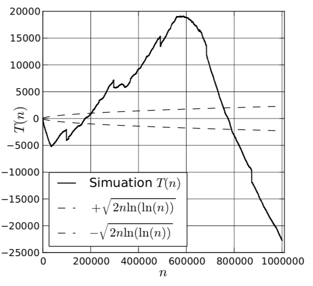
Fig. 19. Simulation results of a simulation model of multiprocessor service.

5.3. Single process statistical model

The main feature of the statistical model is the following: now we use the recurrence equation to accurately calculate the residence time of the application in the system; we process all the data in a single process using a specific Python codebook function; we carry out a certain number of simulations using the Monte Carlo method for better accuracy of calculations. This model gives us “accurate” calculations of the time of application in the system. The main diagram of the model is presented in Figure 20. The student can study the differences between the simulation and statistical models.


Fig. 20. Single process of the statistical model

The program code for implementing the above model is presented in Figure 21. The simulation results are presented in Figure 22.

 #!/usr/bin/python import random import time import numpy as np from numpy import linspace def coroutine(func): del start(*args,**kwargs): g = func(*args,**kwargs) g.next() return g return start def print_header(): "Output rezults - header" f=open("out.txt","w") f.write("%d\n" % N) ##number of points in printing template f.write("%d\n" % TMPN) for t in range(M): f.write("%d%s" % (glambda[t],",")) f.write("%d\n" % glambda[M]) f.close() def print_results(in_seq): "Output rezults" f=open("out.txt","a") k=() for i in range(N-2): if in_seq[i].cid==template[k]: f.write("%f%s" % (in_seq[i].st,",")) k+=1 f.write("%f\n" % (in_seq[N-1 ].st)) f.close() coroutine def server(i): ST=0 ##sojourn time for the previous client item=None while True: item = (yield item) ##get item if item == None: ##new Monte Carlo iteration ST=0 continue waiting_time=max(0.0,ST-item.st-item.tau) item.st+=random.expovariate(glambda[i+1])+waiting_time ST=item.st def producer(): results=[] i=0 while True: if i == N: break c=Client(i,0.,0.) if i!=0: c.tau=random.expovariate(glambda[0]) i+= 1 for s in p: c=s.send(c) results+=[c] for s in p: c=s.send(None) ##final signal return results class Client(object): def __init__(self,cid,st,tau): self.cid=cid self.st=st self.tau=tau def params(self): return (self.cid,self.st,self.tau) stt=time.time() N=1000000 ## Clients M=5 ## Servers ## Input/sevice frequency glambda= [30000]+[i for i in linspace(25000,5000,M)] MKS=20 ## Monte Carlo simulation results ## Number of points in the printing template TMPN=N/10000 ##printing template template= map(int,linspace(0,N-1,TMPN)) print_header() p=[] for i in range(M):p +=[server(i)] for i in range! MKS): print_results(producer()) print("Step=%d" % i) sys.stdout.write("Processing time:%d\n" % int(time.time()-stt)) 

Fig. 21. Python code for a single process statistical model


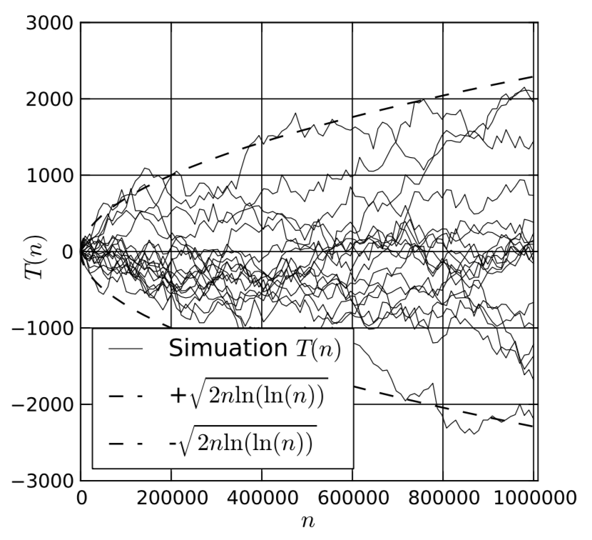
Fig. 22. Simulation results for a single process statistical model

5.4. MPI Statistical Model

The next step in the development of our model is to use the Python MPI module - mpi4py. This allows us to work with a large number of Monte Carlo simulations and use the cluster to run and test the model. The next step should be further development of the model based on the use of the C programming language, “real” MPI or SWIG (https://ru.wikipedia.org/wiki/SWIG) technology for Python. This model is almost identical to the previous model with the only difference that mpi4py is used for multiprocessing and integration of results (Figure 23).


Fig. 23. Statistical MPI Model

In addition to the previous model, several additional modules must be imported. The print_results () function should also be rewritten, since at this stage we have more tests. We must also rewrite the main part of the program. In Figure 24, we provided only the part of the program code that is different from the code of the previous model. The simulation results are presented in Figure 25.

 .................... import sys from mpi4py import MPI .................... def print_results(in_seq): "Output rezults" f=open("out.txt","a") for m in range(int(size)): for j in range(MKS): for i in range(TMPN-l): f.write("%f%s" % (in_seq[m][i+j*TMPN].st,",")) f.write("%f\n" % (in_seq[m][(TMPN-l)+j*TMPN].st)) f.close() .................... stt=time.time() #start time for the process rank = MPI.COMM_WORLD.Get_rank() size = MPI.COMM_WORLD.Get_size() name = MPI.Get_processor_name() N= 10**3 ## Clients M=5 ## Servers ## Input/sevice frequency glambda=[30000]+[i for i in linspace(25000,5000,M)] ## Number of Monte-Carlo simulations for this particuar process MKS=20 TMPN=200 ## Number of points in printing templat template= map(int,linspace(0,N-1,TMPN)) ## points for printing p=[] results=[] ## this process results total_results=[] ## overall results for i in range(M):p +=[server(i)] for i in range(MKS):results+=producer() total_results=MPI.COMM_WORLD.gather(results,0) random.seed(rank) if rank == 0: print_header() print_results(total_results) sys.stdout.write("Processing time: %d\n" % int(time.time()-stt)) 

Fig. 24. Python code for an MPI based statistical model


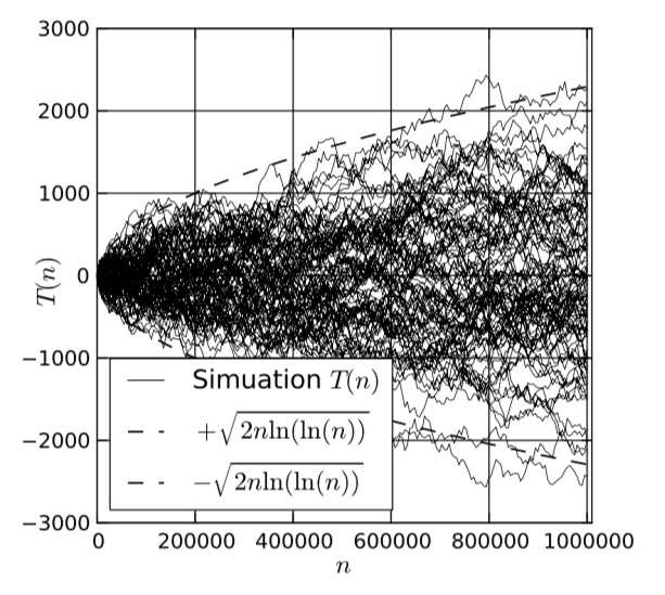
Fig. 25. Simulation results of the statistical MPI model

6. Conclusions

This article has reviewed several models for simulation-based learning. These models enable the student to conduct a series of experiments and increase the understanding of the discipline of Scientific Informatics. There are several levels of complexity of the models presented and experiments with such models. The first level is basic. He brings us to the understanding of random variables, and also gives a primary understanding of the field of scientific research. The next level is more complex and provides a deeper understanding of parallel programming and stochastic modeling. Corresponding theoretical knowledge is presented, and, if necessary, can be used as additional material. This all provides the basic tools for introducing Scientific Informatics. And at the endwe would like to give recommendations for further study and improvement of the models.

6.1. The linearity of the model and the statistical parameters of the QS

The multiphase QS model presented in this article is not linear [12]. This becomes apparent from the recurrence equation, since it contains the nonlinear mathematical function max. If we want to get the correct simulation results, especially in the case of calculating the statistical parameters of the QS, we must use a partially linear model for the calculation. This is especially important for unloaded transport systems, because otherwise we can get a rather large erroneous difference in the calculations.

6.2. Python module extensions and parallel programming with C

For skilled students, it may be interesting to continue improving the efficiency of the code. This can be done by extending Python modules with implemented C functions using SWING technology. It is possible to improve code calculations and speed up computations using Cython, the C programming language, the “real” MPI technology of HTC (high performance computing) in cluster systems [5, 28, 29].

6.3. Efficiency of software solutions and further development

In this section, a student can learn the effectiveness of various software solutions. This topic is important for any software models that are based on parallel computing. The student can study the effectiveness of various software models and try to improve the algorithms step by step. The key point here is the study of the relationship between the number of information flows and calculations for various software processes. So the ratio is important in building the most efficient development of parallel computing programs. Another interesting topic is the study of the possibility of transforming an algorithmic structure into a cluster HTC structure.

As an additional task for research, the authors consider the simulation of QS, which should be modeled and analyzed. The relatively complex nature of QS and the corresponding type of applications require the use of more extensive programming techniques. Thus, there is a good basic platform for implementing such common programming concepts as inheritance, encapsulation, and polymorphism. On the other hand, the basic theoretical concepts of computer science also need to highlight. In addition to all this, the statistical and simulation modeling of QS requires more advanced knowledge in the field of probability theory, the use of more computational resources and the provision of a real scientific computing environment, as well as good motivation of an advanced student.

Literature