Postgres logging experience
We developed our own logging system on PostgreSQL ... Yes, I know that there are add-ons over ElasticSearch (GrayLog2, Logstash), and that there are other similar tools, and there are those about which I don’t know. However, our tool is currently built on PostgreSQL, and it works.
During the working week from all the VLSI services in the cloud, we receive more than 11 billion records per day, they are stored for 3 days, the total amount of space occupied does not exceed 32 TB. All this handles 8 servers with PostgreSQL 9.6. Each server has 24 cores, 16GB RAM and 4 SSDs of 1TB each.

Our services are written in 40% Python, 50% C ++, 9% SQL, 1% Javascript. There are more than 200 services. Often it is necessary to quickly understand the problems of various kinds - the analysis of recorded errors or logical ones. Sometimes you just need to monitor the work, check whether everything goes according to the conceived scenario. All of this can be done by diverse groups: developers, testers, server administrators, and in some cases, management. Therefore, we need a clear tool for all these groups. We have created our own logging system, or, more correctly, a system for tracing http-requests to our web services. It is not a universal solution for logging in general, but it suits our work well. In addition to actually viewing the logs, we have other uses of the data collected - this is the next section.
')
Our http-requests to web-services can be presented in the form of a call tree for convenience of analysis. Simplified this tree can be represented as:
Request for service A
| - Stream Handler Number 1
| | - SQL query to base X
| | - Internal subquery 1
| | | - Request to Redis Y
| | | - Synchronous http request for service B
| | - Internal Subquery 2
| | | - SQL query to base X
| | | - Synchronous http request for service C
| - Stream number 2
| - Asynchronous request for service W
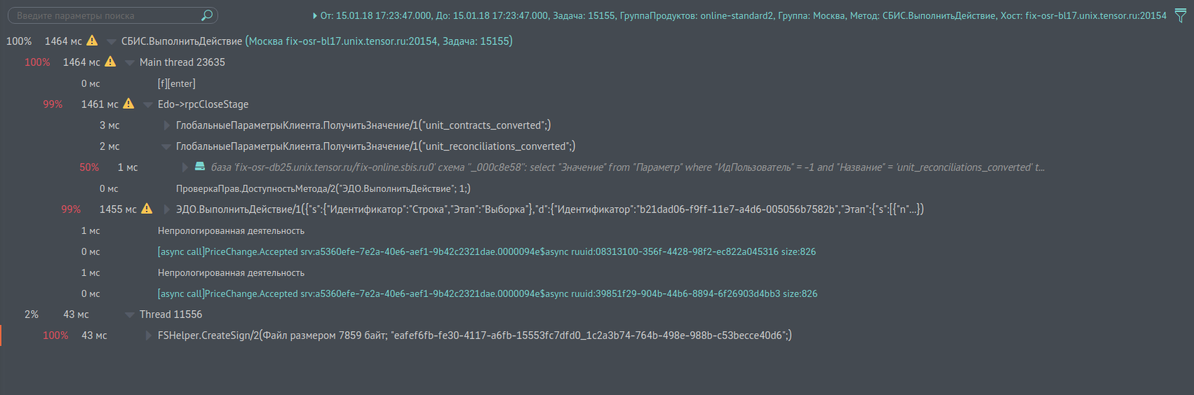
Screen report see fig. 1, representing such a tree, speaks more eloquently. Each node shows how long it took to execute, how many percent it is from the parent. You can search for bottlenecks in the query. On the links you can see the logs of subqueries to other services. The report is quite convenient, it is built almost instantly. There are, of course, exceptions when the call trees contain millions of entries (well, yes, there are such). Here the process takes a little longer, but up to 5 million records in the tree you can get the result. We call this report “single call profiling,” because it is most often used for job profiling.
The image is clickable and opens in the current tab of the web browser.
Fig. 1. Profiling one call
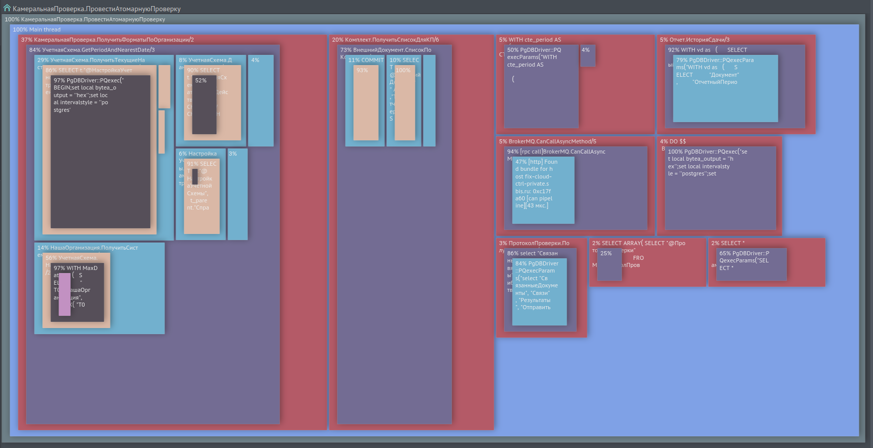
Sometimes there is a need to perform profiling of a typical query on a statistical sample of single-type calls, rather than on a single call. For this we have a report that combines such calls into one tree, showing its nodes and leaves in the form of squares with an area in% of the time of the parent call. See screen in fig. 2
The image is clickable and opens in the current tab of the web browser.
Fig. 2. Profiling by several sample calls
There is a report that allows to detect the presence of network delays. This is when service A sent a request to another service B, the answer was received for 100ms, and the request itself for service B was executed for 10ms, and 90ms disappeared somewhere. This missing time we call the "lag". The screen of the lag report is shown below in fig. 3
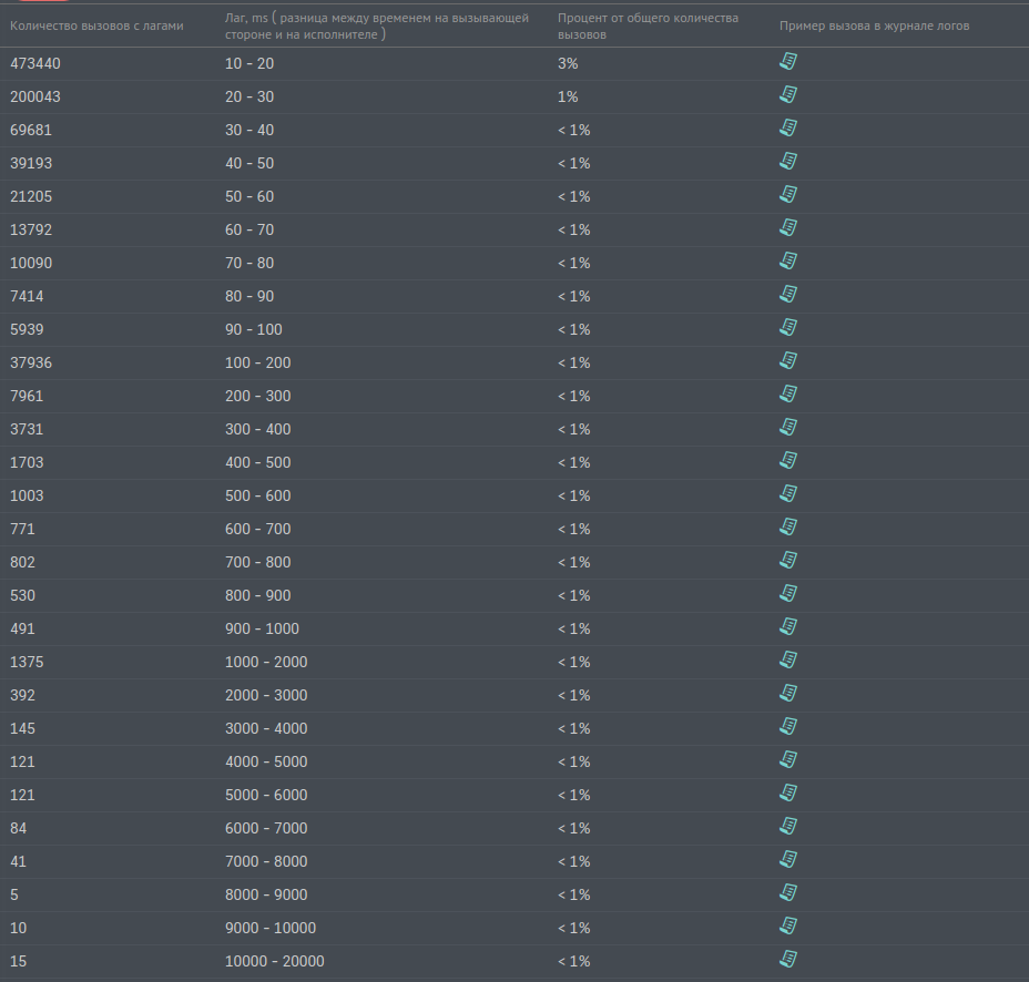
Fig. 3. Report on lags
In addition to these log reports, we use others as well, but they are not as massive as the reports provided.
Our web services are made up of independent peers. Each service node consists of a control process and several workflows. The managing process receives http-requests from the client and puts them in a queue to wait for processing, and also sends responses to the client. Workflows retrieve requests from the control process queue and perform the actual processing. They can access the PostgreSQL database, another web service, or Redis, or somewhere else.
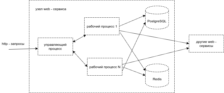
Fig. 4. Process level web service node architecture
Each request to the service has the following set of attributes that we need to write to the logs:
Various events occur within the request: calls to PostgreSQL, Redis, ClickHouse, RabbitMQ, to other services, calls to internal methods of the service. We log these events with the following attributes:
Thus, the data structure looks as a first approximation as in the figure below.
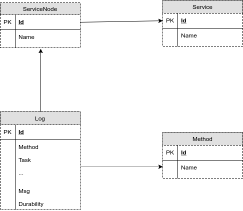
Fig.5. The first version of the structure of the database for storing logs
Here in the picture:
Service - a table with the names of services, there are a few, a few hundred.
ServiceNode - a table with service nodes, it has several thousand entries, several nodes can be associated with one service
Method - a table with the names of the methods, there are also several thousand of them.
Log - Log - actually, the main table where the data of the request and its events are written. The table is intentionally denormalized so as not to waste time on join on large tables in queries and not to keep extra indexes. For example, the query attributes could be placed in a separate table, but then the logic of adding and extracting data would become more complicated. It would have been possible to put out the UUID and User Session Identifier, but would have to have an index on a new table across the field for each such remote field, an index on the foreign key in the Log table and an unnecessary primary key in the new table.
Web services send logs via http, via nginx (for balancing). Log service nodes process them and write to the database. The diagram is shown below.

Fig. 6. Scheme of sending logs to the service logs
Figure 7 shows the screen, what our query logs look like for the fix-osr-bl17.unix.tensor.ru node of the Moscow service. The request is called “VLSI. Perform Action”, its number is 15155. I will not give the UUID, it is displayed above the name of the request. The first one is a record with the message of the form “[m] [start] Edo → EDOCertCheckAttorney” - this is the capture of the event of the start of the call to the internal method of the service without arguments. The next one is immediately followed by the second subquery “[m] [start] Document. Incoming / 1 (234394;)” with one argument with the value 234394. Then it calls the c node of the caching service, this is indicated by the string “[rpc call] ... etc.

The image is clickable and opens in the current tab of the web browser.
Fig. 7. Screen of the log screen using the “BIS. Execute Action” method on the “fix-osr-bl17.unix.tensor.ru” node
For one and a half years of existence, this database and service scheme has not undergone major changes. What problems did we encounter? Initially, we wrote in one database and from the very first days we were faced with the fact that:
These operations quite well dispersed the PostgreSQL server. We tried to change the synchronous_commit and commit_delay parameters, but in our case they did not noticeably affect the performance.
Taking into account the splitting of the tables into the data sections for each day of the month, the new database scheme now looked like this:
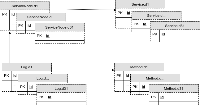
Fig. 8. Diagram of the database with tables for each day of the month.
Over time, with ever-increasing volumes of logs, we could no longer store data in one database. And the first prototype of the log service was altered into a distributed version. Now each node of the logging service wrote to one of several databases, choosing a database for writing using the round-robin algorithm. It was quite comfortable. Statistically, each database received the same load, the load was scaled horizontally, the data volumes on the databases coincided with an accuracy of GB. Instead of a single PostgreSQL server for logs, it now worked. 5. The scheme for the logging service nodes looked like this:

Fig. 9. Scheme of work of the log service with several databases
From the diagram it is clear that each service node keeps connections with several databases. Such a scheme, of course, has drawbacks. If the base failed, or it began to "blunt", then the whole service stopped working, because all were equal to the most recent, well, when adding a new service node, the number of connections to the PostgreSQL server increased.
Simultaneous writing to one table through a large number of connections causes a greater number of locks, which slows down the writing process. With an increase in the number of connections to the base, you can fight using pgBouncer in TRANSACTON MODE. However, miracles do not happen, and in this case the time to fulfill the request increases somewhat, since Still, the work goes through an additional link. Well, with TRANSACTON MODE, the connections to the base are too often switched, which is also not very well reflected in the work.
We have worked on this option for another year, and, finally, switched to a scheme in which one service node works with exactly one database, directly, without pgBouncer. It turned out to be 2 times more efficient, and by that time we added 3 more bases, and we had 8 of them. At that number, we still live to this day.
From this scheme, we have received a small advantage. The number of connections to the database does not grow when a new node is added. If the base starts to blunt, then nginx distributes the load on other nodes of the service.
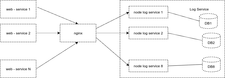
Fig. 10. The current scheme of the service of logs: one node - one base
Additionally, for the best performance of the PostrgeSQL server, and it works for us on Centos 7, we set the deadline scheduler. And they also reduced the size of the dirty cache. This is the vm.dirty_background_bytes parameter, it sets the cache size, upon reaching which the system starts the background process of flushing it to disk. If its volume is too large, the peak load arrives on the disk - the parameter must be selected so that it is smoothed.
In addition to performance problems, there is an acute problem of lack of storage space. Now we are getting around 32 TB. This is enough for the 3rd day. However, sometimes there are peak bursts of logging several times, and the place ends earlier. How to deal with it, without increasing space? We formulated the task for ourselves in the following way: we need at least some logs to remain, even to the detriment of their details.
In accordance with this, we have divided the table of logs for the day into three tables. The first stores data from 0 hours to 8, the second from 8 to 16, the third from 16 to 24. Each of these tables was further divided into three sections. Sections correspond to three levels of logging importance. The first level stores basic information about the fact of the request, its duration, without details, and the facts of errors that occurred during the request. The second level stores information about sub calls and SQL queries. The third level stores everything that is not included in the first two. If the logging service node realizes that less than 15% is left on the record, it starts cleaning the oldest section with the third level. And so on until there is enough space for recording. If there is no more section of the third level, and there is still not enough space, then cleaning of the sections of the second level begins, and at the very least the first, but this has not happened yet.
Before that, it was a question of writing logs, but they make a record in order to read later. In general, for reading, depending on the period of time, the necessary sections of the table are calculated and substituted into the query. The current PostgreSQL mechanism of working with sections is non-working and inconvenient, we do not use it. How the result of the query to the logs looks like, we showed in fig. 7. Basic requirements for the request:
To satisfy both requirements for 100% impossible, but they can be implemented for 80% of requests. This is what we did. It turned out about 20 query profiles that fit into 11 indexes on the Log table. Indexes, unfortunately, slow down the addition of records and steal space. In our variant, these indices take the place comparable to the place for the data.
We never select data for the entire period of time specified by the user to receive the logs, it would be too inefficient. In many cases, displaying the first or last page of a query is sufficient. In more rare cases, users can navigate to the following pages. Consider the algorithm for selecting logs on an example. Let us have requested data for a period of 1 hour with the output of 500 entries on one page:
First we try to build a query for a period of 1 ms in length, turning in parallel to all the databases of the logs. After getting the result from all databases, we merge the query, sorting its data by time. If 500 records are not accumulated, then we shift by 1ms, increase the period by 2 times and repeat the procedure until we collect the necessary 500 records for display.
Most often, this simple algorithm is sufficient for fast data acquisition. But if your filtering conditions are such that millions of records can be selected for the entire period, and among them you need only a few, for example, you are looking for a specific, rarely encountered string in the “Msg” event log field, the result will not be given quickly.
Is everything so bright? Alas, not all ... You can construct a query so that the result does not get for a long time, and fill up with such queries the database server so that they will not be able to work. Since this is used internally, we exclude an intentional blockage - we easily calculate such people, only a random blockage remains. From random we are protected by a timeout on the request, via the PostgreSQL command "SET LOCAL statement_timeout TO ..." The total time of all requests to a single database is given a time of 1200 seconds. The first request to the database is set to 1200 seconds, the second to 1200, less time spent on the first request, etc. If you fail to comply, then an error is returned asking to narrow the filtering conditions.
We made a serious attempt to leave the storage of logs in ClickHouse. Worked with the MergeTree engine. Preliminary tests were excellent, we rolled out the system in preproduction. There were no questions with write speed at all - the gain in storage was up to 7 times. Two nodes ClickHouse processed data, each had 20 cores and 64 GB of memory. By the way, we had PostgreSQL in preproduction a bit more modest in the requirements - 8 cores and 32 GB of memory per server. But be that as it may, the reduction in storage volume in ClickHouse bribed, we were even ready to forgive some degradation of read requests for ClickHouse compared to PostgreSQL.
As soon as the number of requests to the ClickHouse server for data selection became larger than a certain number, they sharply slowed down. We could not defeat it. From ClickHouse had to be abandoned. Perhaps the reason for slowing down the read requests was that you can create only one index on the ClickHouse table. Many profiles of requests to the logs did not fit into this index and data reading was slowed down.
In addition to ClickHouse, they also made a sight on ElasticSearch, they poured data from one PostgreSQL logging database with production (~ 4TB) into it, it gave a gain of about 15% to PostgreSQL at the place of storage in Elastic.
Author: Alexey Terentyev
During the working week from all the VLSI services in the cloud, we receive more than 11 billion records per day, they are stored for 3 days, the total amount of space occupied does not exceed 32 TB. All this handles 8 servers with PostgreSQL 9.6. Each server has 24 cores, 16GB RAM and 4 SSDs of 1TB each.
Who needs it?
Our services are written in 40% Python, 50% C ++, 9% SQL, 1% Javascript. There are more than 200 services. Often it is necessary to quickly understand the problems of various kinds - the analysis of recorded errors or logical ones. Sometimes you just need to monitor the work, check whether everything goes according to the conceived scenario. All of this can be done by diverse groups: developers, testers, server administrators, and in some cases, management. Therefore, we need a clear tool for all these groups. We have created our own logging system, or, more correctly, a system for tracing http-requests to our web services. It is not a universal solution for logging in general, but it suits our work well. In addition to actually viewing the logs, we have other uses of the data collected - this is the next section.
')
Other logging uses
Our http-requests to web-services can be presented in the form of a call tree for convenience of analysis. Simplified this tree can be represented as:
Request for service A
| - Stream Handler Number 1
| | - SQL query to base X
| | - Internal subquery 1
| | | - Request to Redis Y
| | | - Synchronous http request for service B
| | - Internal Subquery 2
| | | - SQL query to base X
| | | - Synchronous http request for service C
| - Stream number 2
| - Asynchronous request for service W
Screen report see fig. 1, representing such a tree, speaks more eloquently. Each node shows how long it took to execute, how many percent it is from the parent. You can search for bottlenecks in the query. On the links you can see the logs of subqueries to other services. The report is quite convenient, it is built almost instantly. There are, of course, exceptions when the call trees contain millions of entries (well, yes, there are such). Here the process takes a little longer, but up to 5 million records in the tree you can get the result. We call this report “single call profiling,” because it is most often used for job profiling.
The image is clickable and opens in the current tab of the web browser.
Fig. 1. Profiling one call
Sometimes there is a need to perform profiling of a typical query on a statistical sample of single-type calls, rather than on a single call. For this we have a report that combines such calls into one tree, showing its nodes and leaves in the form of squares with an area in% of the time of the parent call. See screen in fig. 2
The image is clickable and opens in the current tab of the web browser.
Fig. 2. Profiling by several sample calls
There is a report that allows to detect the presence of network delays. This is when service A sent a request to another service B, the answer was received for 100ms, and the request itself for service B was executed for 10ms, and 90ms disappeared somewhere. This missing time we call the "lag". The screen of the lag report is shown below in fig. 3
Fig. 3. Report on lags
In addition to these log reports, we use others as well, but they are not as massive as the reports provided.
How does it all work
Our web services are made up of independent peers. Each service node consists of a control process and several workflows. The managing process receives http-requests from the client and puts them in a queue to wait for processing, and also sends responses to the client. Workflows retrieve requests from the control process queue and perform the actual processing. They can access the PostgreSQL database, another web service, or Redis, or somewhere else.
Fig. 4. Process level web service node architecture
Each request to the service has the following set of attributes that we need to write to the logs:
- unique name of the request, we call it "service method"
- service node where the request is finally received
- Requestor IP
- user session ID
- UUID of the cascade of requests (the cascade of requests is when one request outside the service generates a series of requests to other services)
- request number on the service node - when the service is restarted, the request numbers are reset
- the number of the workflow that processed the request
Various events occur within the request: calls to PostgreSQL, Redis, ClickHouse, RabbitMQ, to other services, calls to internal methods of the service. We log these events with the following attributes:
- the date and time of the occurrence of the event with an accuracy of milliseconds
- event text is the most important part, everything that does not fit into other attributes is recorded in it: SQL query text, Redis call command, call parameters from another service, asynchronous call parameters via RabbitMQ, etc.
- event duration in milliseconds
- the thread number in which the event occurred
- processor ticks - needed to determine the sequence of events that have the same date and time, the accuracy is up to milliseconds
- event type: normal, warning or error
Thus, the data structure looks as a first approximation as in the figure below.
Fig.5. The first version of the structure of the database for storing logs
Here in the picture:
Service - a table with the names of services, there are a few, a few hundred.
ServiceNode - a table with service nodes, it has several thousand entries, several nodes can be associated with one service
Method - a table with the names of the methods, there are also several thousand of them.
Log - Log - actually, the main table where the data of the request and its events are written. The table is intentionally denormalized so as not to waste time on join on large tables in queries and not to keep extra indexes. For example, the query attributes could be placed in a separate table, but then the logic of adding and extracting data would become more complicated. It would have been possible to put out the UUID and User Session Identifier, but would have to have an index on a new table across the field for each such remote field, an index on the foreign key in the Log table and an unnecessary primary key in the new table.
Web services send logs via http, via nginx (for balancing). Log service nodes process them and write to the database. The diagram is shown below.
Fig. 6. Scheme of sending logs to the service logs
Figure 7 shows the screen, what our query logs look like for the fix-osr-bl17.unix.tensor.ru node of the Moscow service. The request is called “VLSI. Perform Action”, its number is 15155. I will not give the UUID, it is displayed above the name of the request. The first one is a record with the message of the form “[m] [start] Edo → EDOCertCheckAttorney” - this is the capture of the event of the start of the call to the internal method of the service without arguments. The next one is immediately followed by the second subquery “[m] [start] Document. Incoming / 1 (234394;)” with one argument with the value 234394. Then it calls the c node of the caching service, this is indicated by the string “[rpc call] ... etc.
The image is clickable and opens in the current tab of the web browser.
Fig. 7. Screen of the log screen using the “BIS. Execute Action” method on the “fix-osr-bl17.unix.tensor.ru” node
For one and a half years of existence, this database and service scheme has not undergone major changes. What problems did we encounter? Initially, we wrote in one database and from the very first days we were faced with the fact that:
- We will not be able to write to the database in the usual way via INSERT, and we have moved only to the instructions COPY.
- Delete obsolete data in the usual way through DELETE is unrealistic, and we switched to TRUNCATE. This instruction acts fairly quickly on the entire table, truncating the file to almost zero size. However, we had to get our table-section for each day of the month so that only irrelevant data was deleted. With TRUNCATE, there is still one unpleasant moment - if the PostgreSQL server decided to run the autovacuum to prevent wraparound process on the tablet, then TRUNCATE will not run until autovacuum to prevent wraparound is running out, but it can work for quite a while. Therefore, we clean this process before cleaning.
- We do not need a transaction log - and we began to create tables through CREATE UNLOGGED.
- Synchronous writing to disk is not needed - and we did fsync = off and full_page_writes = off, this is acceptable, there were, of course, database outages due to the disks, but they are extremely rare.
These operations quite well dispersed the PostgreSQL server. We tried to change the synchronous_commit and commit_delay parameters, but in our case they did not noticeably affect the performance.
Taking into account the splitting of the tables into the data sections for each day of the month, the new database scheme now looked like this:
Fig. 8. Diagram of the database with tables for each day of the month.
Over time, with ever-increasing volumes of logs, we could no longer store data in one database. And the first prototype of the log service was altered into a distributed version. Now each node of the logging service wrote to one of several databases, choosing a database for writing using the round-robin algorithm. It was quite comfortable. Statistically, each database received the same load, the load was scaled horizontally, the data volumes on the databases coincided with an accuracy of GB. Instead of a single PostgreSQL server for logs, it now worked. 5. The scheme for the logging service nodes looked like this:
Fig. 9. Scheme of work of the log service with several databases
From the diagram it is clear that each service node keeps connections with several databases. Such a scheme, of course, has drawbacks. If the base failed, or it began to "blunt", then the whole service stopped working, because all were equal to the most recent, well, when adding a new service node, the number of connections to the PostgreSQL server increased.
Simultaneous writing to one table through a large number of connections causes a greater number of locks, which slows down the writing process. With an increase in the number of connections to the base, you can fight using pgBouncer in TRANSACTON MODE. However, miracles do not happen, and in this case the time to fulfill the request increases somewhat, since Still, the work goes through an additional link. Well, with TRANSACTON MODE, the connections to the base are too often switched, which is also not very well reflected in the work.
We have worked on this option for another year, and, finally, switched to a scheme in which one service node works with exactly one database, directly, without pgBouncer. It turned out to be 2 times more efficient, and by that time we added 3 more bases, and we had 8 of them. At that number, we still live to this day.
From this scheme, we have received a small advantage. The number of connections to the database does not grow when a new node is added. If the base starts to blunt, then nginx distributes the load on other nodes of the service.
Fig. 10. The current scheme of the service of logs: one node - one base
Additionally, for the best performance of the PostrgeSQL server, and it works for us on Centos 7, we set the deadline scheduler. And they also reduced the size of the dirty cache. This is the vm.dirty_background_bytes parameter, it sets the cache size, upon reaching which the system starts the background process of flushing it to disk. If its volume is too large, the peak load arrives on the disk - the parameter must be selected so that it is smoothed.
In addition to performance problems, there is an acute problem of lack of storage space. Now we are getting around 32 TB. This is enough for the 3rd day. However, sometimes there are peak bursts of logging several times, and the place ends earlier. How to deal with it, without increasing space? We formulated the task for ourselves in the following way: we need at least some logs to remain, even to the detriment of their details.
In accordance with this, we have divided the table of logs for the day into three tables. The first stores data from 0 hours to 8, the second from 8 to 16, the third from 16 to 24. Each of these tables was further divided into three sections. Sections correspond to three levels of logging importance. The first level stores basic information about the fact of the request, its duration, without details, and the facts of errors that occurred during the request. The second level stores information about sub calls and SQL queries. The third level stores everything that is not included in the first two. If the logging service node realizes that less than 15% is left on the record, it starts cleaning the oldest section with the third level. And so on until there is enough space for recording. If there is no more section of the third level, and there is still not enough space, then cleaning of the sections of the second level begins, and at the very least the first, but this has not happened yet.
Before that, it was a question of writing logs, but they make a record in order to read later. In general, for reading, depending on the period of time, the necessary sections of the table are calculated and substituted into the query. The current PostgreSQL mechanism of working with sections is non-working and inconvenient, we do not use it. How the result of the query to the logs looks like, we showed in fig. 7. Basic requirements for the request:
- he should be as fast as possible
- the result of the query should be navigation
To satisfy both requirements for 100% impossible, but they can be implemented for 80% of requests. This is what we did. It turned out about 20 query profiles that fit into 11 indexes on the Log table. Indexes, unfortunately, slow down the addition of records and steal space. In our variant, these indices take the place comparable to the place for the data.
We never select data for the entire period of time specified by the user to receive the logs, it would be too inefficient. In many cases, displaying the first or last page of a query is sufficient. In more rare cases, users can navigate to the following pages. Consider the algorithm for selecting logs on an example. Let us have requested data for a period of 1 hour with the output of 500 entries on one page:
First we try to build a query for a period of 1 ms in length, turning in parallel to all the databases of the logs. After getting the result from all databases, we merge the query, sorting its data by time. If 500 records are not accumulated, then we shift by 1ms, increase the period by 2 times and repeat the procedure until we collect the necessary 500 records for display.
Most often, this simple algorithm is sufficient for fast data acquisition. But if your filtering conditions are such that millions of records can be selected for the entire period, and among them you need only a few, for example, you are looking for a specific, rarely encountered string in the “Msg” event log field, the result will not be given quickly.
Is everything so bright? Alas, not all ... You can construct a query so that the result does not get for a long time, and fill up with such queries the database server so that they will not be able to work. Since this is used internally, we exclude an intentional blockage - we easily calculate such people, only a random blockage remains. From random we are protected by a timeout on the request, via the PostgreSQL command "SET LOCAL statement_timeout TO ..." The total time of all requests to a single database is given a time of 1200 seconds. The first request to the database is set to 1200 seconds, the second to 1200, less time spent on the first request, etc. If you fail to comply, then an error is returned asking to narrow the filtering conditions.
Attempts to go to other log storage systems
We made a serious attempt to leave the storage of logs in ClickHouse. Worked with the MergeTree engine. Preliminary tests were excellent, we rolled out the system in preproduction. There were no questions with write speed at all - the gain in storage was up to 7 times. Two nodes ClickHouse processed data, each had 20 cores and 64 GB of memory. By the way, we had PostgreSQL in preproduction a bit more modest in the requirements - 8 cores and 32 GB of memory per server. But be that as it may, the reduction in storage volume in ClickHouse bribed, we were even ready to forgive some degradation of read requests for ClickHouse compared to PostgreSQL.
As soon as the number of requests to the ClickHouse server for data selection became larger than a certain number, they sharply slowed down. We could not defeat it. From ClickHouse had to be abandoned. Perhaps the reason for slowing down the read requests was that you can create only one index on the ClickHouse table. Many profiles of requests to the logs did not fit into this index and data reading was slowed down.
In addition to ClickHouse, they also made a sight on ElasticSearch, they poured data from one PostgreSQL logging database with production (~ 4TB) into it, it gave a gain of about 15% to PostgreSQL at the place of storage in Elastic.
Author: Alexey Terentyev
Source: https://habr.com/ru/post/347222/
All Articles