Generative Modeling and AI
In the previous chapter, we talked about classical discriminative models in machine learning and dismantled the simplest examples of such models. Let's now look at the bigger picture.
Artificial Intelligence (AI) is an algorithm that can solve problems that are typically solved by people, at a level comparable or superior to human. This can be the recognition of visual images, understanding and analysis of texts, control mechanisms and the construction of logical chains. An artificial intelligence system is a system that can effectively solve all such tasks at once. The solution to this problem still does not exist, but there are various approaches that can be called the first steps towards solving the problem of AI.
In the twentieth century, the rule-based approach was the most popular. His idea is that the world obeys laws that, for example, physics and other natural sciences are studying. And even if they cannot be effectively programmed in AI directly, it is reasonable to assume that with a sufficient number of programmed rules, an AI system based on computers can effectively exist in a world based on these rules and solve arbitrary tasks. This approach does not take into account the natural stochasticity of some events. To take it into account, it is necessary to construct a probabilistic model on this list of rules for making stochastic decisions, provided random input data are available.
')
A full description of the world would require such a large number of rules that it is impossible to set and maintain them manually. Hence the idea to conduct enough observations of events in the real world and derive the necessary rules automatically from these observations. This idea immediately supports both the actual stochasticity of some natural processes, as well as the imaginary stochasticity, arising from the fact that it is not fully known what factors influence a certain deterministic process. An automatic derivation of the rules from observations is done by a section of mathematics called machine learning, and it is this that is currently the most promising foundation for AI.
In the previous chapter, we looked at the classical machine learning problems (classification and regression) and the classical linear methods for solving them (logistic and linear regression). In reality, for complex problems, nonlinear models are used, usually based either on decision trees or on deep artificial neural networks, which are better shown for processing dense data with a high level of redundancy: images, sound and text.
These methods are capable of automatically deriving rules based on observations, and they are very successfully applied in commercial applications. However, they have a disadvantage, because of which they are insufficient for use as an AI system - they are specifically designed to solve a specific, highly specialized task, for example, to distinguish cats and dogs in an image. Obviously, a model that summarizes an image into a single number loses a lot of data. To determine the cat on the image does not necessarily understand the essence of the cat, you just need to learn how to look for the main features of this cat. The task of classifying an image does not imply a complete understanding of the scene, but only a search for specific objects in it. It is not possible to determine the classifier for all possible combinations of connections for all possible combinations of objects, if only because of the exponentially large amount of observations that need to be collected and marked. Therefore, the ideas of classical problems of machine learning with reinforcement, in which a specific task is solved, are not suitable. For AI, a fundamentally different approach to the formulation of the problem for machine learning is needed.
So, we need, having a set of observations, in a sense, to understand the process that generates them. We reformulate this problem in a probabilistic language. Let observation be the realization of a random variable. and there is a set of observed events
 , i = \ overline {1, N} \}% 0") . Then the “understanding” of the whole variety of events can be formulated as the task of restoring the distribution
. Then the “understanding” of the whole variety of events can be formulated as the task of restoring the distribution % 0") .
.
There are several approaches to solving this problem. One of the most common methods is the introduction of a latent variable. Let's say there is some kind of representation% 0") observations
observations  . This presentation describes the “understanding” of the observation model. For example, for the frame of a computer game such an understanding can be the relevant state of the game world and the position of the camera. In this case
  = \ int_Z P (x | z) P (z) dz% 0") . Fixing
. Fixing % 0") so that it is easy to sample the distribution, we get a model in which
so that it is easy to sample the distribution, we get a model in which % 0") and
and % 0") you can bring neural networks. Teaching this model with standard deep learning methods can be obtained according to the formula above, after which we can use it in probabilistic inference. More precise formulations of such models will be in the subsequent parts, but here it should be noted that complex versions of such models require approximation of complex noncomputable integrals, for which approximate methods are usually used, such as MCMC or Variational Inference . Building to extract samples from it is called the task of generative modeling.
you can bring neural networks. Teaching this model with standard deep learning methods can be obtained according to the formula above, after which we can use it in probabilistic inference. More precise formulations of such models will be in the subsequent parts, but here it should be noted that complex versions of such models require approximation of complex noncomputable integrals, for which approximate methods are usually used, such as MCMC or Variational Inference . Building to extract samples from it is called the task of generative modeling.
You can approach the question differently. In fact, explicitly count , approximating complex integrals is not necessary. One idea is that if a model can “imagine” the world for itself, then it understands how it works. For example, if I can draw a person in different positions and angles, then I understand how his anatomy and perspective as a whole are arranged. If people cannot distinguish objects generated by a model from real ones, then the model has been able to honestly “understand” how this or that phenomenon works as well as these people understand it. This idea inspires the development of generative modeling with implicit - development of models, which, having a finite number of observations, are able to generalize them and generate new observations that are indistinguishable from real ones. Let's pretend that % 0") , or any other simple sampling distribution. Then, under fairly general conditions, there is a function
, or any other simple sampling distribution. Then, under fairly general conditions, there is a function  such that
  \ sim P (x)% 0") . In this case, we do not get explicitly, but the model still contains information about it implicitly. Instead of recovering can recover
. In this case, we do not get explicitly, but the model still contains information about it implicitly. Instead of recovering can recover % 0") followed by samples from can be obtained as
followed by samples from can be obtained as , z \ sim N (0,1)% 0") . cannot be used in probabilistic output directly, but, firstly, it is not always necessary, and secondly, when it is needed, you can often use Monte Carlo methods, for which you just need to get samples. The methods of this type include the Generative Adversarial Networks model, which is explored in the next section.
. cannot be used in probabilistic output directly, but, firstly, it is not always necessary, and secondly, when it is needed, you can often use Monte Carlo methods, for which you just need to get samples. The methods of this type include the Generative Adversarial Networks model, which is explored in the next section.
Let's look at a simple generative model. Let there be some observable value% 0") . For example, it can be a person's height or a pixel image. Suppose that this value is fully explained by some hidden (latent) value . In our analogy, this may be the weight of a person or an object and its orientation in an image. Suppose now that for a hidden quantity
. For example, it can be a person's height or a pixel image. Suppose that this value is fully explained by some hidden (latent) value . In our analogy, this may be the weight of a person or an object and its orientation in an image. Suppose now that for a hidden quantity  = N (z; 0, 1)% 0") , and the observed value depends linearly with normal noise, i.e.
, and the observed value depends linearly with normal noise, i.e.  = N (x; Wz + b, \ sigma ^ 2 I)% 0") . This model is called Probabilistic Principal Component Analysis (PPCA) and, in essence, it is a probabilistic reformulation of the classical Principal Component Analysis (PCA) model, in which the visible variable linearly dependent on latent variable
. This model is called Probabilistic Principal Component Analysis (PPCA) and, in essence, it is a probabilistic reformulation of the classical Principal Component Analysis (PCA) model, in which the visible variable linearly dependent on latent variable  no noise.
Expectation Maximization (EM) - an algorithm for training models with latent variables. Details can be found in the specialized literature, but the general essence of the algorithm is quite simple:
If the M-step does not maximize the likelihood to the end, but only take a step in the direction of the maximum, it is called Generalized EM (GEM).
Let us apply to our PCA EM model an algorithm and a maximum likelihood method for finding optimal parameters.% 0") models. The joint likelihood of the observed and latent parameters can be written as:
models. The joint likelihood of the observed and latent parameters can be written as:
 = \ log P (x | \ theta) = \ log P (x | \ theta) \ int_z q (z) = \ int_z q (z) \ log P (x | \ theta)% 0")
Where% 0") - this is an arbitrary distribution. Next, we will omit the conditional distribution of the parameters in order to facilitate the formulas.
- this is an arbitrary distribution. Next, we will omit the conditional distribution of the parameters in order to facilitate the formulas.
 \ log P (x | \ theta) = \ int_z q (z) \ log \ frac {P (x, z)} {P (z | x)} = \ int_z q (z) \ log \ frac {P (x, z) q (z)} {q (z) P (z | x)} =")
 \ logP (x, z) - \ int_zq (z) \ logq (z) + \ int_zq (z) \ log \ frac {q (z)} {P (z | x)} =")
 \ log P (x, z) + H \ left (q \ left (z \ right) \ right) + KL (q (z) || P (z | x))% 0")
Where is the value || P (z | x)) = \ int_z q (z) \ log \ frac {q (z)} {P (z | x)}") called
called  divergence between distributions and . Magnitude
  \ right) = - \ int_z q (z) \ log q (z)") called entropy .
called entropy .  \ right)") independent of parameters
independent of parameters  , so we can ignore this addend when optimizing:
 \ propto \ int_z q (z) \ log P (x, z) + KL (q (z) || P (z | x)) =")
 \ log \ left (P (x | z) P (z) \ right) + KL (q (z) || P (z | x)) =")
 \ log P (x | z) + \ int_z q (z) \ log P (z) + KL (q (z) || P (z | x)) \ propto")
 \ log P (x | z) + KL (q (z) || P (z | x))")
Magnitude || P (z | x))") non-negative and zero when
non-negative and zero when  = P (z | x)") . In this regard, let's define the following EM algorithm:
. In this regard, let's define the following EM algorithm:
PPCA is a linear model, because it can be solved analytically. But instead, we will try to solve it with the help of a generalized EM-algorithm, when maximization is performed not up to the end, but only by one step of the gradient rise in the direction of the optimum. Moreover, we will use a stochastic gradient lift, i.e. his step will be a step towards optimum only on average. Since our data is iid,
 \ propto \ int_z q (z) \ log P (x | z) = \ int_z q (z) \ log \ prod_ {i = 1} ^ {N} P (x_i | z_i) = \ int_z q (z) \ sum_ {i = 1} ^ {N} \ log P (x_i | z_i)")
Note that the expression of the form f (z)") is a mathematical expectation
is a mathematical expectation } f (z)") . Then
. Then
 \ sum_ {i = 1} ^ {N} \ log P (x_i | z_i) = E_ {z \ sim q (z)} \ sum_ {i = 1} ^ {N} \ log P (x_i | z_i) \ propto E_ {z \ sim q (z)} \ frac {1} {N} \ sum_ {i = 1} ^ {N} \ log P (x_i | z_i)")
Since a single sample is an unbiased estimate of the expectation, the following equality can be written approximately:
} \ frac {1} {N} \ sum_ {i = 1} ^ {N} \ log P (x_i | z_i) = \ frac {1} {N} \ sum_ {i = 1} ^ {N} \ log P (x_i | z_i)")
Total by substituting , we get:
 \ propto \ frac {1} {N} \ sum_ {i = 1} ^ {N} \ log P (x_i | z_i) =")
 ^ d \ left | \ sigma ^ 2 I \ right |}} \ exp \ left (- \ frac {{|| x_i - \ left (W z_i + b \ right) ||} ^ 2} {2 \ sigma ^ 2} \ right) \ right ) =")
 ^ d} } \ exp \ left (- \ frac {{|| x_i - \ left (W z_i + b \ right) ||} ^ 2} {2 \ sigma ^ 2} \ right) \ right) =")
 ^ d} - \ frac {1 } {2 \ sigma ^ 2} {|| x_i - b - W z_i ||} ^ 2 \ right)")
or
 \ propto L ^ {*} (x | \ theta) = - \ frac {1} {N} \ sum_ {i = 1} ^ {N} \ left (d \ log \ left ( \ sigma ^ 2 \ right) + \ frac {1} {\ sigma ^ 2} {|| x_i - b - W z_i ||} ^ 2 \ right)")
Formula 1. Loss function proportional to the likelihood of data in the PPCA model.
Where - dimension of the observed variable . Now let's write out the GEM-algorithm for PPCA. , but
  = N \ left (z; \ left (W ^ TW + \ sigma ^ 2 I \ right) ^ {- 1} W ^ T \ left (x - b \ right), \ sigma ^ 2 \ left (W ^ TW + \ sigma ^ 2 I \ right) ^ {- 1} \ right)") . Then the GEM algorithm will look like this:
. Then the GEM algorithm will look like this:
After the model is trained, samples can be generated from it:
 = N (x; b, W W ^ T + \ sigma ^ 2 I)")
Let's train the PPCA model using standard SGD. We will again study the work of the model on a toy example in order to understand all the details. The full model code can be found here , and in this article only key points will be covered.
Set = N (x; \ left (\ begin {matrix} 5 \\ 10 \ end {matrix} \ right) \ left (\ begin {matrix} 1.2 ^ 2 & 0 \\ 0 & 2.4 ^ 2 \ end {matrix} \ right))") - two-dimensional normal distribution with a diagonal covariance matrix. - one-dimensional normal latent view.
- two-dimensional normal distribution with a diagonal covariance matrix. - one-dimensional normal latent view.

Fig. 1. Ellipse around the middle, which falls 95% of the points from the distribution .
So the first thing to do is generate the data. We generate samples from :
Now you need to determine the parameters of the model:
After that you can get their latent views for the sample of visible variables:
Here you need to pay attention to tf.stop_gradient (...). This function does not allow the parameter values within the input subgraph to affect the gradient by these parameters. It is necessary that: = P (z | x)") remained fixed during the M-step, which is necessary for the correct operation of the EM algorithm.
remained fixed during the M-step, which is necessary for the correct operation of the EM algorithm.
Let's write down the loss function now.") for optimization at M-step:
for optimization at M-step:
So, the model is ready for training. Let's take a look at the learning curve of the model:
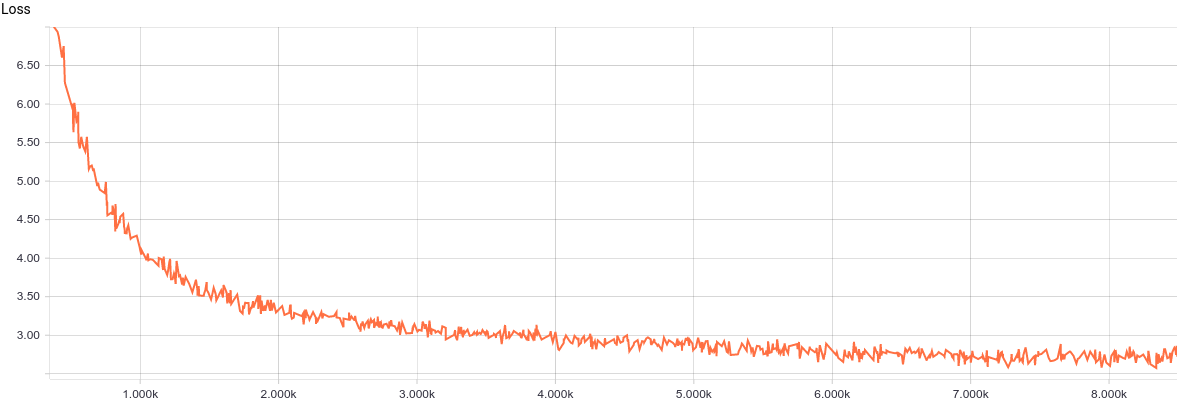
Fig. 2. The PPCA learning curve.
It can be seen that the model converges fairly regularly and quickly, which well reflects the simplicity of the model. Let's look at the learned distribution parameters.

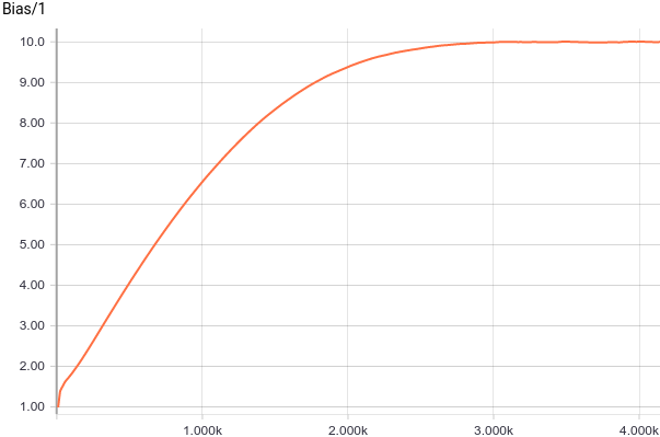
Fig. 3. Displacement plots from the origin (parameter ).
).
It's clear that quickly converged to analytical values
  and
and  . Let's now look at the parameters.
  :
:

Fig. 4. Graph of parameter change .
.
See that the value converged to 1.2, i.e. to the smaller axis of deviation of the input distribution, as expected.
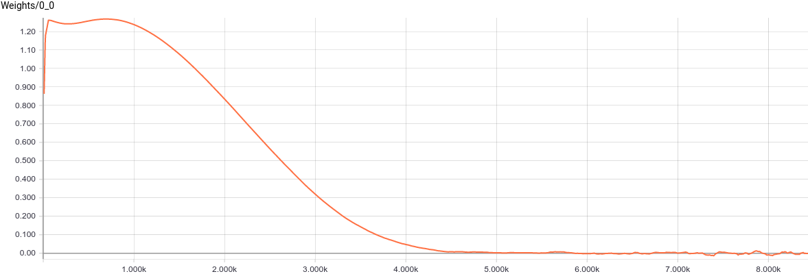
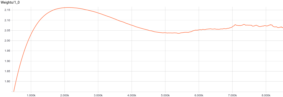
Fig. 5. Graphs of parameters change .
.
 , in turn, came to about the value at which
  . Substituting these values into the model, we get
  that means we restored the distribution of the data.
Let's look at the distribution of data. The latent variable is one-dimensional, because it is displayed as a one-dimensional distribution. The visible variable is two-dimensional, but its given covariance matrix is diagonal, which means that its ellipsoid is aligned with the axes of coordinates. Therefore, we will display it as two projections of its distribution on the coordinate axes. This is the set and learned distribution. in projection on the first axis of coordinates:
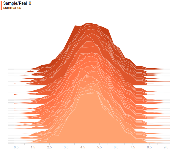
Fig. 6. The projection of a given distribution on the first axis of coordinates.
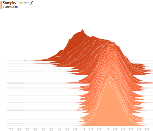
Fig. 7. Projection of the learned distribution") on the first axis of coordinates.
on the first axis of coordinates.
And this is the set and learned distribution. projected on the second axis of coordinates:
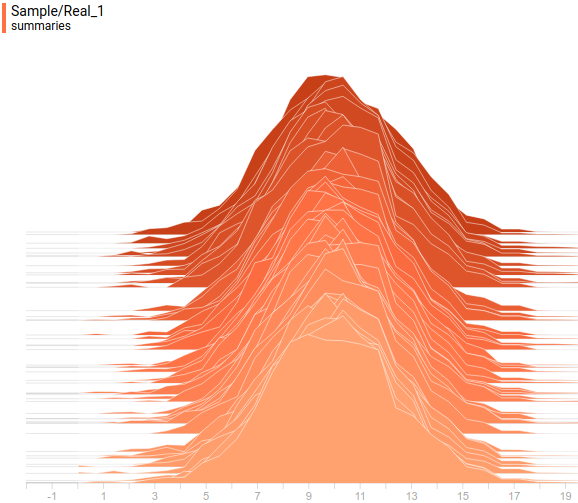
Fig. 8. The projection of a given distribution on the second axis of coordinates.
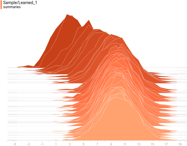
Fig. 9. Projection of the learned distribution on the second axis of coordinates.
And so look analytic and learned distribution :
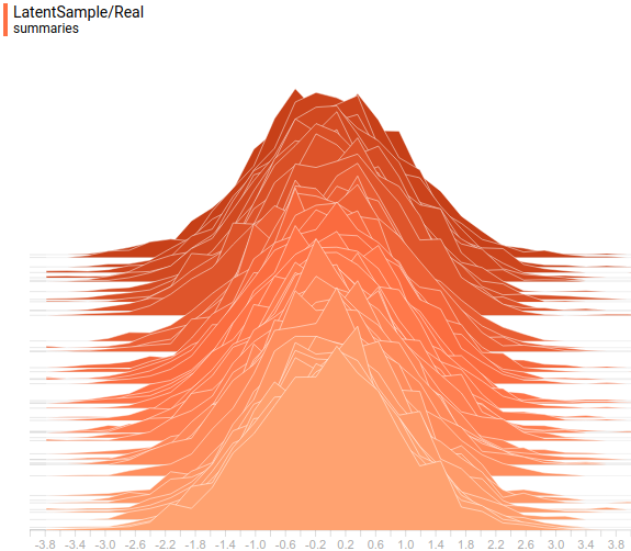
Fig. 10. Specified distribution .
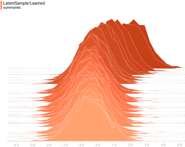
Fig. 11. Learned distribution") .
.
It can be seen that all the distributions learned converge to distributions very similar to those given by the task. Let's look at the dynamics of the training model, to be sure of this finally:
Fig. 12. The training process of the PPCA model, in which the learned distribution converges to data distribution .
The presented model is a probabilistic interpretation of the classical PCA model, which is a linear model. We used the math from the original article , built the GEM algorithm on top of it and showed that the resulting model converges to an analytical solution using a simple example. Of course, if in the problem it was not normal, the model would not have done so well. In the same way as PCA does not cope perfectly with data that does not lie in a certain hyperplane. To solve more complex problems of approximating distributions, we need more complex and nonlinear models. One of these models, Generative Adversarial Networks, will be discussed in the next article.
Thank you Olga Talanova for reviewing the text. Thanks to Andrei Tarashkevich for help with the layout of this article.
Artificial Intelligence Task
Artificial Intelligence (AI) is an algorithm that can solve problems that are typically solved by people, at a level comparable or superior to human. This can be the recognition of visual images, understanding and analysis of texts, control mechanisms and the construction of logical chains. An artificial intelligence system is a system that can effectively solve all such tasks at once. The solution to this problem still does not exist, but there are various approaches that can be called the first steps towards solving the problem of AI.
In the twentieth century, the rule-based approach was the most popular. His idea is that the world obeys laws that, for example, physics and other natural sciences are studying. And even if they cannot be effectively programmed in AI directly, it is reasonable to assume that with a sufficient number of programmed rules, an AI system based on computers can effectively exist in a world based on these rules and solve arbitrary tasks. This approach does not take into account the natural stochasticity of some events. To take it into account, it is necessary to construct a probabilistic model on this list of rules for making stochastic decisions, provided random input data are available.
')
A full description of the world would require such a large number of rules that it is impossible to set and maintain them manually. Hence the idea to conduct enough observations of events in the real world and derive the necessary rules automatically from these observations. This idea immediately supports both the actual stochasticity of some natural processes, as well as the imaginary stochasticity, arising from the fact that it is not fully known what factors influence a certain deterministic process. An automatic derivation of the rules from observations is done by a section of mathematics called machine learning, and it is this that is currently the most promising foundation for AI.
AI machine trained
In the previous chapter, we looked at the classical machine learning problems (classification and regression) and the classical linear methods for solving them (logistic and linear regression). In reality, for complex problems, nonlinear models are used, usually based either on decision trees or on deep artificial neural networks, which are better shown for processing dense data with a high level of redundancy: images, sound and text.
These methods are capable of automatically deriving rules based on observations, and they are very successfully applied in commercial applications. However, they have a disadvantage, because of which they are insufficient for use as an AI system - they are specifically designed to solve a specific, highly specialized task, for example, to distinguish cats and dogs in an image. Obviously, a model that summarizes an image into a single number loses a lot of data. To determine the cat on the image does not necessarily understand the essence of the cat, you just need to learn how to look for the main features of this cat. The task of classifying an image does not imply a complete understanding of the scene, but only a search for specific objects in it. It is not possible to determine the classifier for all possible combinations of connections for all possible combinations of objects, if only because of the exponentially large amount of observations that need to be collected and marked. Therefore, the ideas of classical problems of machine learning with reinforcement, in which a specific task is solved, are not suitable. For AI, a fundamentally different approach to the formulation of the problem for machine learning is needed.
Probabilistic formulation of the problem of understanding the world
So, we need, having a set of observations, in a sense, to understand the process that generates them. We reformulate this problem in a probabilistic language. Let observation be the realization of a random variable.
and there is a set of observed events . Then the “understanding” of the whole variety of events can be formulated as the task of restoring the distribution .There are several approaches to solving this problem. One of the most common methods is the introduction of a latent variable. Let's say there is some kind of representation
observations . This presentation describes the “understanding” of the observation model. For example, for the frame of a computer game such an understanding can be the relevant state of the game world and the position of the camera. In this case . Fixing so that it is easy to sample the distribution, we get a model in which and you can bring neural networks. Teaching this model with standard deep learning methods can be obtained according to the formula above, after which we can use it in probabilistic inference. More precise formulations of such models will be in the subsequent parts, but here it should be noted that complex versions of such models require approximation of complex noncomputable integrals, for which approximate methods are usually used, such as MCMC or Variational Inference . Building to extract samples from it is called the task of generative modeling.You can approach the question differently. In fact, explicitly count
, approximating complex integrals is not necessary. One idea is that if a model can “imagine” the world for itself, then it understands how it works. For example, if I can draw a person in different positions and angles, then I understand how his anatomy and perspective as a whole are arranged. If people cannot distinguish objects generated by a model from real ones, then the model has been able to honestly “understand” how this or that phenomenon works as well as these people understand it. This idea inspires the development of generative modeling with implicit - development of models, which, having a finite number of observations, are able to generalize them and generate new observations that are indistinguishable from real ones. Let's pretend that , or any other simple sampling distribution. Then, under fairly general conditions, there is a function such that . In this case, we do not get explicitly, but the model still contains information about it implicitly. Instead of recovering can recover followed by samples from can be obtained as . cannot be used in probabilistic output directly, but, firstly, it is not always necessary, and secondly, when it is needed, you can often use Monte Carlo methods, for which you just need to get samples. The methods of this type include the Generative Adversarial Networks model, which is explored in the next section.Principal component analysis
Let's look at a simple generative model. Let there be some observable value
. For example, it can be a person's height or a pixel image. Suppose that this value is fully explained by some hidden (latent) value . In our analogy, this may be the weight of a person or an object and its orientation in an image. Suppose now that for a hidden quantity , and the observed value depends linearly with normal noise, i.e. . This model is called Probabilistic Principal Component Analysis (PPCA) and, in essence, it is a probabilistic reformulation of the classical Principal Component Analysis (PCA) model, in which the visible variable linearly dependent on latent variable no noise.Expectation Maximization
Expectation Maximization (EM) - an algorithm for training models with latent variables. Details can be found in the specialized literature, but the general essence of the algorithm is quite simple:
- Initialize the model with initial parameter values.
- E-step. Fill in the latent variables with their expected values in the current model.
- M-pitch. Maximize the likelihood of a model with fixed values of latent variables. For example, gradient descent on the parameters.
- Repeat (2, 3) until the expected values of the latent variables stop changing.
If the M-step does not maximize the likelihood to the end, but only take a step in the direction of the maximum, it is called Generalized EM (GEM).
PCA Solution with EM
Let us apply to our PCA EM model an algorithm and a maximum likelihood method for finding optimal parameters.
models. The joint likelihood of the observed and latent parameters can be written as:Where
- this is an arbitrary distribution. Next, we will omit the conditional distribution of the parameters in order to facilitate the formulas.Where is the value
called divergence between distributions and . Magnitude called entropy . independent of parameters , so we can ignore this addend when optimizing:Magnitude
non-negative and zero when . In this regard, let's define the following EM algorithm:- E: . This will nullify the second term. .
- M: Maximize the first term
 \ propto \ int_z q (z) \ log P (x | z)") .
.
PPCA is a linear model, because it can be solved analytically. But instead, we will try to solve it with the help of a generalized EM-algorithm, when maximization is performed not up to the end, but only by one step of the gradient rise in the direction of the optimum. Moreover, we will use a stochastic gradient lift, i.e. his step will be a step towards optimum only on average. Since our data is iid,
Note that the expression of the form
is a mathematical expectation . ThenSince a single sample is an unbiased estimate of the expectation, the following equality can be written approximately:
Total by substituting
, we get:or
Formula 1. Loss function proportional to the likelihood of data in the PPCA model.
Where
- dimension of the observed variable . Now let's write out the GEM-algorithm for PPCA. , but . Then the GEM algorithm will look like this:- Initialize the parameters
 reasonable random initial approximations.
 - Sampling
") - selection of the mini-batches from the data.
- selection of the mini-batches from the data. - Calculate the expected values of latent variables.
") or
or  ^ {- 1} W ^ T \ left (x_i - b \ right) + \ varepsilon, \ varepsilon \ sim N (0, \ sigma ^ 2 \ left (W ^ TW + \ sigma ^ 2 I \ right) ^ {- 1})") .
. - Substitute
 in formula (1) for and take a step gradient rise in the parameters. It is important to remember that
  must be taken as inputs and not allowed to propagate the error back inside it.
 - If the likelihood of the data and the expected values of the latent variables for the control visible variables do not change much, stop learning. Otherwise, go to step (2).
After the model is trained, samples can be generated from it:
Numerical solution of the PCA problem
Let's train the PPCA model using standard SGD. We will again study the work of the model on a toy example in order to understand all the details. The full model code can be found here , and in this article only key points will be covered.
Set
- two-dimensional normal distribution with a diagonal covariance matrix. - one-dimensional normal latent view.Fig. 1. Ellipse around the middle, which falls 95% of the points from the distribution
.So the first thing to do is generate the data. We generate samples from
:def normal_samples(batch_size): def example(): return tf.contrib.distributions.MultivariateNormalDiag( [5, 10], [1.2, 2.4]).sample(sample_shape=[1])[0] return tf.contrib.data.Dataset.from_tensors([0.]) .repeat() .map(lambda x: example()) .batch(batch_size) Now you need to determine the parameters of the model:
input_size = 2 latent_space_size = 1 stddev = tf.get_variable( "stddev", initializer=tf.constant(0.1, shape=[1])) biases = tf.get_variable( "biases", initializer=tf.constant(0.1, shape=[input_size])) weights = tf.get_variable( "Weights", initializer=tf.truncated_normal( [input_size, latent_space_size], stddev=0.1)) After that you can get their latent views for the sample of visible variables:
def get_latent(visible, latent_space_size, batch_size): matrix = tf.matrix_inverse( tf.matmul(weights, weights, transpose_a=True) + stddev**2 * tf.eye(latent_space_size)) mean_matrix = tf.matmul(matrix, weights, transpose_b=True) # Multiply each vector in a batch by a matrix. expected_latent = batch_matmul( mean_matrix, visible - biases, batch_size) stddev_matrix = stddev**2 * matrix noise = tf.contrib.distributions.MultivariateNormalFullCovariance( tf.zeros(latent_space_size), stddev_matrix) .sample(sample_shape=[batch_size]) return tf.stop_gradient(expected_latent + noise) Here you need to pay attention to tf.stop_gradient (...). This function does not allow the parameter values within the input subgraph to affect the gradient by these parameters. It is necessary that
remained fixed during the M-step, which is necessary for the correct operation of the EM algorithm.Let's write down the loss function now.
for optimization at M-step: sample = dataset.get_next() latent_sample = get_latent(sample, latent_space_size, batch_size) norm_squared = tf.reduce_sum((sample - biases - batch_matmul(weights, latent_sample, batch_size))**2, axis=1) loss = tf.reduce_mean( input_size * tf.log(stddev**2) + 1/stddev**2 * norm_squared) train = tf.train.AdamOptimizer(learning_rate) .minimize(loss, var_list=[bias, weights, stddev], name="train") So, the model is ready for training. Let's take a look at the learning curve of the model:
Fig. 2. The PPCA learning curve.
It can be seen that the model converges fairly regularly and quickly, which well reflects the simplicity of the model. Let's look at the learned distribution parameters.
Fig. 3. Displacement plots from the origin (parameter
).It's clear that
quickly converged to analytical values and . Let's now look at the parameters. :Fig. 4. Graph of parameter change
.See that the value
converged to 1.2, i.e. to the smaller axis of deviation of the input distribution, as expected.Fig. 5. Graphs of parameters change
. , in turn, came to about the value at which . Substituting these values into the model, we get that means we restored the distribution of the data.Let's look at the distribution of data. The latent variable is one-dimensional, because it is displayed as a one-dimensional distribution. The visible variable is two-dimensional, but its given covariance matrix is diagonal, which means that its ellipsoid is aligned with the axes of coordinates. Therefore, we will display it as two projections of its distribution on the coordinate axes. This is the set and learned distribution.
in projection on the first axis of coordinates:Fig. 6. The projection of a given distribution
on the first axis of coordinates.Fig. 7. Projection of the learned distribution
on the first axis of coordinates.And this is the set and learned distribution.
projected on the second axis of coordinates:Fig. 8. The projection of a given distribution
on the second axis of coordinates.Fig. 9. Projection of the learned distribution
on the second axis of coordinates.And so look analytic and learned distribution
:Fig. 10. Specified distribution
.Fig. 11. Learned distribution
.It can be seen that all the distributions learned converge to distributions very similar to those given by the task. Let's look at the dynamics of the training model, to be sure of this finally:
Fig. 12. The training process of the PPCA model, in which the learned distribution
converges to data distribution .Conclusion
The presented model is a probabilistic interpretation of the classical PCA model, which is a linear model. We used the math from the original article , built the GEM algorithm on top of it and showed that the resulting model converges to an analytical solution using a simple example. Of course, if in the problem
it was not normal, the model would not have done so well. In the same way as PCA does not cope perfectly with data that does not lie in a certain hyperplane. To solve more complex problems of approximating distributions, we need more complex and nonlinear models. One of these models, Generative Adversarial Networks, will be discussed in the next article.Thanks
Thank you Olga Talanova for reviewing the text. Thanks to Andrei Tarashkevich for help with the layout of this article.
Source: https://habr.com/ru/post/347184/
All Articles