Calculation snuffled modern rocket engines
Introduction
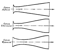
The rocket engine nozzle is a technical device that serves to accelerate the gas flow passing through it to speeds exceeding the speed of sound. The main types of nozzle profiles are shown in the figure:
')
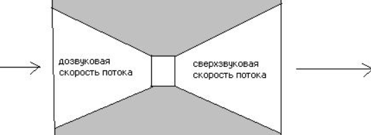
Due to the high efficiency of the gas flow acceleration, Laval nozzles have found practical application. The nozzle is a channel narrowed in the middle. In the simplest case, such a nozzle may consist of a pair of truncated cones, conjugated by narrow ends:
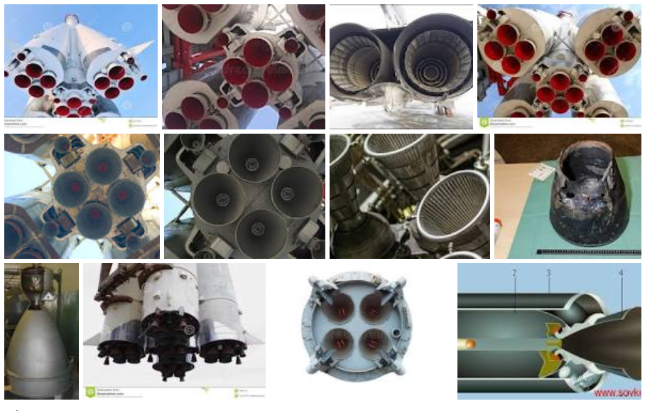
In the rocket engine the Laval nozzle was first used by General M. M. Pomortsev in 1915. In November 1915, General MM Pomortsev addressed the Aerodynamic Institute with a draft pneumatic missile.
Pomortseva rocket was set in motion by compressed air, which significantly limited its range, but it made it noiseless. The rocket was intended for firing from the trenches at enemy positions. Warhead was equipped with TNT.
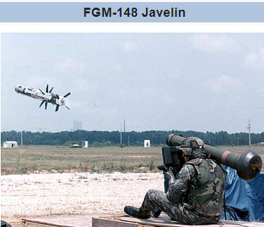
In the Pomortsev rocket, two interesting constructive solutions were applied: there was a Laval nozzle in the engine, and a ring stabilizer was connected to the body. Similar constructions are used at the present time, but already with a solid-fuel engine and an automatic guidance system:
However, the problems remained old, but in a modern version: a limited range of up to 3 km., Targeting and holding the target in good visibility, which is not real for a real battle, not protected from electromagnetic obstructions and, last but not least, high price.
Theoretical basis
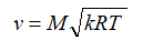
Efficient nozzles of modern rocket engines are profiled on the basis of special gas-dynamic calculations. The basic equation relating the gradient of the sectional area, the velocity gradient and the Mach number is as follows:
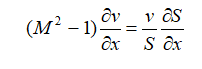
where: S is the nozzle section area; v is the gas velocity; M is the Mach number (the ratio of the gas velocity at any point in the stream to the speed of sound at the same point).
Analyzing this ratio, we find that the following flow regimes can be implemented in the Laval nozzle:
1) M <1 - subsonic input stream: [1]
but)
 <0, then
  > 0 (from equation). Subsonic flow in a narrowing channel accelerates.
b)
> 0, then <0. Subsonic flow in an expanding channel is inhibited.2) M> 1 is the supersonic inlet flow:
but)
<0, then <0. Supersonic flow in a narrowing channel is inhibited.b)
> 0, then > 0 The supersonic flow in the expanding channel accelerates.3)
= 0 - the narrowest point of the nozzle, the minimum section.Then either M = 1 is possible (the flow passes through the speed of sound), or
= 0 (speed extremum).Which of the modes is implemented in practice depends on the pressure difference between the nozzle inlet and the environment.
If the pressure reached in the critical section exceeds the external pressure, then the flow at the nozzle exit will be supersonic. Otherwise, it remains subsonic. [2]
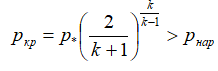 - supersonic outflow condition.
where: p * is the braking pressure (pressure in the chamber); pcr - pressure in the nozzle throat; pnar - pressure in the environment; k is the adiabatic index.
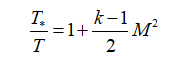
If the parameters in the combustion chamber are known, then the parameters in any section of the nozzle can be recognized by the following relationships:
pressure:
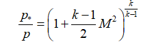 or
or 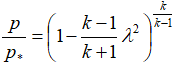 ;
;temperature:
 or
or 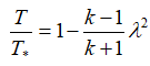 ;
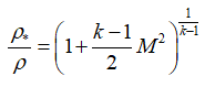
;density:
 or
or 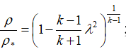 ;
;speed:
 or
or 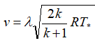 .
.In these formulas, λ is the superficial velocity, the ratio of the gas velocity in a given nozzle section to the speed of sound in the critical section, R is the specific gas constant. The index "*" denotes the braking parameters (in this case, the parameters in the combustion chamber).
Formulation of the problem
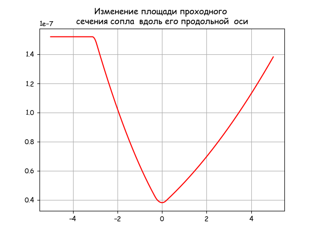
1. To calculate the parameters of the flow of gases in the Laval nozzle: for this, the profile of the Laval nozzle is divided into 150 control points -
 . The splitting is carried out in such a way that the minimum section is located at
  . The values of the gas-dynamic functions of pressure, density and temperature in each section are determined.
2. Perform calculations using high-level freely distributed Python programming language according to the following calculation scheme and source data:
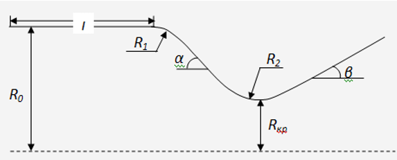
Figure 1: Laval nozzle profile
Table 1-Baseline
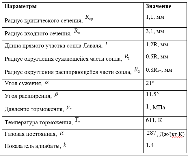
The given initial data are of a demonstration nature.
Calculation of the Laval nozzle by means of Python
Listing to build a profile and square bore of a Laval nozzle
#!/usr/bin/env python #coding=utf8 import matplotlib.pyplot as plt import matplotlib as mpl mpl.rcParams['font.family'] = 'fantasy' mpl.rcParams['font.fantasy'] = 'Comic Sans MS, Arial' import numpy as np from math import * alfa=21.0# beta=11.5# rkr=1.1# R0=2*rkr r1=0.5*rkr# r2=0.8*rkr# ye=rkr+r2 L=1.2*R0# x0=0 y0=R0 xa=L ya=y0 xc1=xa yc1=ya-r1 xc=xa+r1*cos(radians(90-alfa)) yc=yc1+r1*sin(radians(90-alfa)) yd=ye-r2*sin(radians(90-alfa)) xd=xc+(yc-yd)/tan(radians(alfa)) xc2=xd+r2*sin(radians(alfa)) xe=xc2 xf=xe+r2*cos(radians(90-beta)) yf=ye-r2*sin(radians(90-beta)) def R(x): if x0<=x<=xa: return ya*1e-4 if xa<=x<=xc: return (yc1+sqrt(r1**2-(x-xc1)**2))*1e-4 if xc<=x<=xd: return (-tan(radians(alfa))*(x-xc)+yc)*1e-4 if xd<=x<=xf: return (ye-sqrt(r2**2-(x-xe)**2))*1e-4 if xf<=x: return (yf+tan(radians(beta))*(x-xf))*1e-4 y=[R(x+xe) for x in np.arange(-5,5,0.01)] x=np.arange(-5,5,0.01) plt.figure() plt.title(' ') plt.axis([-5.0, 5.0, 0.0, 3.0*10**-4]) plt.plot(x,y,'r') plt.grid(True) plt.figure() plt.title(' \n ') yy=[pi*R(x+xe)**2 for x in np.arange(-5,5,0.01)] plt.plot(x,yy,'r') plt.grid(True) plt.show() 
To continue solving the problem in Python, you need to associate λ - the reduced gas velocity with the x coordinate along the longitudinal axis. For this, I used the fsolve function from the SciPy library with the following instruction:
fsolve (<function>, <starting point>, xtol = 1.5 · 10 ^ 8)
I give a fragment of the program for managing the solver with one starting point:
def lamda(z): m=round(Q(z),2) if z>= 0: x=fsolve(lambda x:x*( (1-(1/6)*x**2)**2.5)/((1-(1/6))**2.5)-m,1.5) return x[0] if z<0: x=fsolve(lambda x:x*( (1-(1/6)*x**2)**2.5)/((1-(1/6))**2.5)-m,0.5) return x[0] This is the only possible Python solution to a complex algebraic equation with a power function of the adiabatic exponent k. For example, even for a simplified equation using the SymPy library, we get an invalid calculation time for only one point:
from sympy import * import time x = symbols('x',real=True) start = time.time() start = time.time() d=solve( 1.5774409656148784068*x *(1.0-0.16666666666666666667*x**2)**2.5-0.25,x) stop = time.time() print (" :",round(stop-start,3)) print(round(d[0],3)) print(round(d[1],3)) Solver working time: 195.675
0.16
1.95
Listing for calculating relative velocity gas dynamic function
#!/usr/bin/env python #coding=utf8 import matplotlib.pyplot as plt import matplotlib as mpl mpl.rcParams['font.family'] = 'fantasy' mpl.rcParams['font.fantasy'] = 'Comic Sans MS, Arial' import numpy as np from math import * from scipy.optimize import * import time start = time.time() alfa=21.0# beta=11.5# rkr=1.1# R0=2*rkr r1=0.5*rkr# r2=0.8*rkr# ye=rkr+r2 L=1.2*R0# x0=0 y0=R0 xa=L ya=y0 xc1=xa yc1=ya-r1 xc=xa+r1*cos(radians(90-alfa)) yc=yc1+r1*sin(radians(90-alfa)) yd=ye-r2*sin(radians(90-alfa)) xd=xc+(yc-yd)/tan(radians(alfa)) xc2=xd+r2*sin(radians(alfa)) xe=xc2 xf=xe+r2*cos(radians(90-beta)) yf=ye-r2*sin(radians(90-beta)) def R(x): if x0<=x<=xa: return ya*1e-4 if xa<=x<=xc: return (yc1+sqrt(r1**2-(x-xc1)**2))*1e-4 if xc<=x<=xd: return (-tan(radians(alfa))*(x-xc)+yc)*1e-4 if xd<=x<=xf: return (ye-sqrt(r2**2-(x-xe)**2))*1e-4 if xf<=x: return (yf+tan(radians(beta))*(x-xf))*1e-4 def S(x): return pi*R(x+xe)**2 xg=2*xe n=150 RG=287 # Tt=611 # k=1.4 def tau(x): return 1-(1/6)*x**2 def eps(x): return (1-(1/6)*x**2)**2.5 def pip(x): return 1-(1/6)*x**2 def Q(z): return S(0)/S(z) x=[x0-xe+(i/n)*(xg-x0) for i in np.arange(0,n,1)] def lamda(z): m=round(Q(z),2) if z>= 0: x=fsolve(lambda x:x*( (1-(1/6)*x**2)**2.5)/((1-(1/6))**2.5)-m,1.5) return x[0] if z<0: x=fsolve(lambda x:x*( (1-(1/6)*x**2)**2.5)/((1-(1/6))**2.5)-m,0.5) return x[0] plt.title(' ') y=[lamda(z) for z in x] stop = time.time() print (" :",round(stop-start,3)) plt.ylabel('λ(xi)- ' ) plt.plot(0, 1, color='b', linestyle=' ', marker='o', label=' ') plt.xlabel('xi - ') plt.plot(x,y,'r') plt.legend(loc='best') plt.grid(True) plt.show() Program working time: 0.222
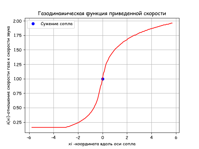
Conclusion:
The plot of the distribution of velocities of the gas stream is fully consistent with the above theory. At the same time, according to the proposed algorithm and library, the calculation time at 150 points is 1000 times less than for one point using solve sympy.
Listing for calculating the gas-dynamic function of temperature
#!/usr/bin/env python #coding=utf8 import matplotlib.pyplot as plt import matplotlib as mpl mpl.rcParams['font.family'] = 'fantasy' mpl.rcParams['font.fantasy'] = 'Comic Sans MS, Arial' import numpy as np from math import * from scipy.optimize import * import time start = time.time() alfa=21.0# beta=11.5# rkr=1.1# R0=2*rkr r1=0.5*rkr# r2=0.8*rkr# ye=rkr+r2 L=1.2*R0# x0=0 y0=R0 xa=L ya=y0 xc1=xa yc1=ya-r1 xc=xa+r1*cos(radians(90-alfa)) yc=yc1+r1*sin(radians(90-alfa)) yd=ye-r2*sin(radians(90-alfa)) xd=xc+(yc-yd)/tan(radians(alfa)) xc2=xd+r2*sin(radians(alfa)) xe=xc2 xf=xe+r2*cos(radians(90-beta)) yf=ye-r2*sin(radians(90-beta)) def R(x): if x0<=x<=xa: return ya*1e-4 if xa<=x<=xc: return (yc1+sqrt(r1**2-(x-xc1)**2))*1e-4 if xc<=x<=xd: return (-tan(radians(alfa))*(x-xc)+yc)*1e-4 if xd<=x<=xf: return (ye-sqrt(r2**2-(x-xe)**2))*1e-4 if xf<=x: return (yf+tan(radians(beta))*(x-xf))*1e-4 def S(x): return pi*R(x+xe)**2 xg=2*xe n=150 RG=287 # Tt=611 # k=1.4 def tau(x): return 1-(1/6)*x**2 def eps(x): return (1-(1/6)*x**2)**2.5 def pip(x): return 1-(1/6)*x**2 def Q(z): return S(0)/S(z) x=[x0-xe+(i/n)*(xg-x0) for i in np.arange(0,n,1)] def lamda(z): m=round(Q(z),2) if z>= 0: x=fsolve(lambda x:x*( (1-(1/6)*x**2)**2.5)/((1-(1/6))**2.5)-m,1.5) return x[0] if z<0: x=fsolve(lambda x:x*( (1-(1/6)*x**2)**2.5)/((1-(1/6))**2.5)-m,0.5) return x[0] plt.title(' ') t0=293 y=[ t0*tau(lamda(z)) for z in x] stop = time.time() print (" :",round(stop-start,3)) plt.ylabel('T(xi)- . ' ) plt.xlabel('xi - ') plt.plot(x,y,'r') plt.grid(True) plt.show() Program working time: 0.203
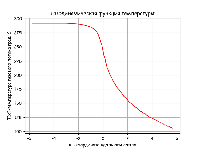
Conclusion
The temperature at the nozzle exit decreases according to the equation of gas dynamics given in the listing. The program execution time is acceptable - 0.203 .
Test setup:
Listing to calculate the gas-dynamic pressure function
#!/usr/bin/env python #coding=utf8 import matplotlib.pyplot as plt import matplotlib as mpl mpl.rcParams['font.family'] = 'fantasy' mpl.rcParams['font.fantasy'] = 'Comic Sans MS, Arial' import numpy as np from math import * from scipy.optimize import * import time start = time.time() alfa=21.0# beta=11.5# rkr=1.1# R0=2*rkr r1=0.5*rkr# r2=0.8*rkr# ye=rkr+r2 L=1.2*R0# x0=0 y0=R0 xa=L ya=y0 xc1=xa yc1=ya-r1 xc=xa+r1*cos(radians(90-alfa)) yc=yc1+r1*sin(radians(90-alfa)) yd=ye-r2*sin(radians(90-alfa)) xd=xc+(yc-yd)/tan(radians(alfa)) xc2=xd+r2*sin(radians(alfa)) xe=xc2 xf=xe+r2*cos(radians(90-beta)) yf=ye-r2*sin(radians(90-beta)) def R(x): if x0<=x<=xa: return ya*1e-4 if xa<=x<=xc: return (yc1+sqrt(r1**2-(x-xc1)**2))*1e-4 if xc<=x<=xd: return (-tan(radians(alfa))*(x-xc)+yc)*1e-4 if xd<=x<=xf: return (ye-sqrt(r2**2-(x-xe)**2))*1e-4 if xf<=x: return (yf+tan(radians(beta))*(x-xf))*1e-4 def S(x): return pi*R(x+xe)**2 xg=2*xe n=150 RG=287 # Tt=611 # k=1.4 def tau(x): return 1-(1/6)*x**2 def eps(x): return (1-(1/6)*x**2)**2.5 def pip(x): return 1-(1/6)*x**2 def Q(z): return S(0)/S(z) x=[x0-xe+(i/n)*(xg-x0) for i in np.arange(0,n,1)] def lamda(z): m=round(Q(z),2) if z>= 0: x=fsolve(lambda x:x*( (1-(1/6)*x**2)**2.5)/((1-(1/6))**2.5)-m,1.5) return x[0] if z<0: x=fsolve(lambda x:x*( (1-(1/6)*x**2)**2.5)/((1-(1/6))**2.5)-m,0.5) return x[0] plt.title(' ') p0=3.6 y=[ 3.6*pip(lamda(z)) for z in x] stop = time.time() print (" :",round(stop-start,3)) plt.ylabel('P(xi)- ' ) plt.xlabel('xi - ') plt.plot(x,y,'r') plt.grid(True) plt.show() Program working time: 0.203
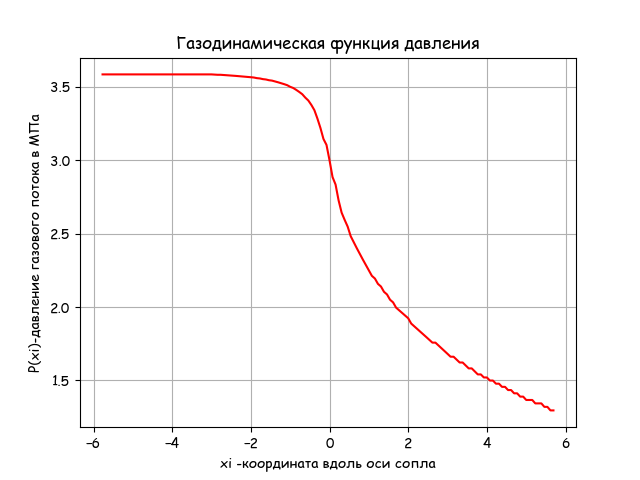
Conclusion
The pressure at the nozzle outlet decreases according to the gas dynamics equation given in the listing. Program execution time is acceptable -0.203.
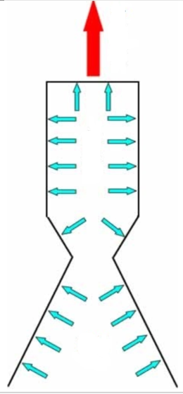
The occurrence of thrust from the action of gas pressure is shown schematically in the figure:
Listing to calculate the gas-dynamic function of the relative density of the gas
#!/usr/bin/env python #coding=utf8 import matplotlib.pyplot as plt import matplotlib as mpl mpl.rcParams['font.family'] = 'fantasy' mpl.rcParams['font.fantasy'] = 'Comic Sans MS, Arial' import numpy as np from math import * from scipy.optimize import * import time start = time.time() alfa=21.0# beta=11.5# rkr=1.1# R0=2*rkr r1=0.5*rkr# r2=0.8*rkr# ye=rkr+r2 L=1.2*R0# x0=0 y0=R0 xa=L ya=y0 xc1=xa yc1=ya-r1 xc=xa+r1*cos(radians(90-alfa)) yc=yc1+r1*sin(radians(90-alfa)) yd=ye-r2*sin(radians(90-alfa)) xd=xc+(yc-yd)/tan(radians(alfa)) xc2=xd+r2*sin(radians(alfa)) xe=xc2 xf=xe+r2*cos(radians(90-beta)) yf=ye-r2*sin(radians(90-beta)) def R(x): if x0<=x<=xa: return ya*1e-4 if xa<=x<=xc: return (yc1+sqrt(r1**2-(x-xc1)**2))*1e-4 if xc<=x<=xd: return (-tan(radians(alfa))*(x-xc)+yc)*1e-4 if xd<=x<=xf: return (ye-sqrt(r2**2-(x-xe)**2))*1e-4 if xf<=x: return (yf+tan(radians(beta))*(x-xf))*1e-4 def S(x): return pi*R(x+xe)**2 xg=2*xe n=150 RG=287 # Tt=611 # k=1.4 def tau(x): return 1-(1/6)*x**2 def eps(x): return (1-(1/6)*x**2)**2.5 def pip(x): return 1-(1/6)*x**2 def Q(z): return S(0)/S(z) x=[x0-xe+(i/n)*(xg-x0) for i in np.arange(0,n,1)] def lamda(z): m=round(Q(z),2) if z>= 0: x=fsolve(lambda x:x*( (1-(1/6)*x**2)**2.5)/((1-(1/6))**2.5)-m,1.5) return x[0] if z<0: x=fsolve(lambda x:x*( (1-(1/6)*x**2)**2.5)/((1-(1/6))**2.5)-m,0.5) return x[0] plt.title(' ') y=[ eps(lamda(z)) for z in x] stop = time.time() print (" :",round(stop-start,3)) plt.ylabel(' ' ) plt.xlabel('xi - ') plt.plot(x,y,'r') plt.grid(True) plt.show() Program working time: 0.203
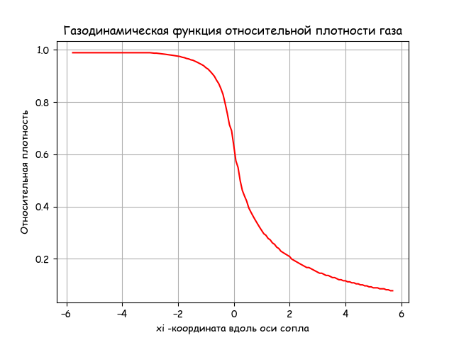
Conclusion
The gas density at the nozzle exit decreases according to the gas dynamics equation given in the listing. Program execution time is acceptable.
findings
- A method for solving the real roots of nonlinear power equations with fractional exponents used to describe gas-dynamic processes using Python tools has been developed. The method is based on the use of the fsolve solver from the scipy module. optimize.
- With the help of the developed method, the demo problem of calculating the nozzle of modern rocket engines has been solved with the definition of the following gas-dynamic functions: speed; temperatures; pressure; reactive gas densities.
Links
1. A. A. Dorofeev, Fundamentals of the Theory of Thermal Rocket Engines (General Theory of Rocket Engines) MSTU. N. E. Bauman Moscow 1999
2. Landau, LD, Lifshits, E. M. Chapter X. One-dimensional motion of a compressible gas. § 97. Gas outflow through a nozzle // Theoretical Physics. - T. 6. Hydrodynamics.
Source: https://habr.com/ru/post/347086/
All Articles