Mobile devices from the inside. The image structure of partitions containing the file system. Part 2

The image structure of partitions containing the file system. Part 2.

Start publishing, read in Part 1.

3.2._sparsechunk files

Since Although the sparse file, although it is a compressed source data file, can also be quite large, its modification appeared, called _sparsechunk files, which is the same sparse file, but cut into smaller pieces based on a previously selected borders (according to the file cutting algorithm).

This add-on allows you to use compressed sparse files to transfer updates via OTA or download in fastboot mode.

3.2.1.Structure of _sparsechunk-files

By structure, each _sparsechunk file is a regular sparse file, but containing not all, but only a part of the input file, for example, a partition image. The size of this part is compressed, i.e. in a sparse view, must not exceed a predetermined value or boundary. Currently, the "border" size _sparsechunk file, is usually 256MB ( 268,435,456 bytes).
')
The next part of the sparse file is contained in the next _sparsechunk file, etc.

Externally, these files are distinguished by an index in the name, which determines the sequence of their processing during decoding. The index may simply be an ordinal number or may be represented as an offset in the input file up to a chunk.

So First, the image of the section is encoded into a sparse file, and then converted (cut) into a set of _sparsechunk files.

The process of creating a _sparsechunk file can be described by the following algorithm:

1. The finished sparse file is viewed and all consecutive pieces (chunks) of the Raw and Fill types are grouped into a group called “data”, the length of which is constantly monitored. The procedure is performed until the group size reaches the limit, the value of which is indicated in advance and is determined by the requirements listed above when describing the file splitting process;
2. If the joining of the next piece leads to exceeding the border, then it is not included in the group, and a separate file is formed from the already grouped pieces, to which a piece of the DontCare type, called “final”, is added, in which the data offset to the end of the output file is specified in the Chunk_Size field. This file is named _sparsechunk.1;
3. The sparse file continues to be searched according to the method of paragraphs 1–2 and the next _sparsechunk file is formed; just before its formation, a sparse DontCare piece , called “initial”, is added to the sparse group of pieces in front of which the data offset is specified in the Chunk_Size field, contained in this file, from the beginning of the original image. At the end of the “final” piece is added, formed by the above algorithm;
4. This continues until the end of the sparse file is reached.

Thus, each _sparsechunk file can consist of three parts, which I have named:

1. OFFSET_TO_START - contains the "initial" piece;
2. INFO - the part containing the "data";
3. OFFSET_TO_END - contains the "final" piece.

The OFFSET_TO_START part is an offset in the input file before the beginning of the “data” part that contains information in the sparse form.

The INFO part contains only information in a sparse form, consisting of sparse pieces of the type Fill and Raw .

The OFFSET_TO_END part is the offset to the end of the output file. If the offset is zero, i.e. if the _sparsechunk file containing the info group is the last in the set of _sparsechunk files, then the OFFSET_TO_END part is completely absent.

3.2.2. Working with _sparsechunk files

As an example of working with _sparsechunk files, let's look at the conversion of _sparsechunk files into a sparse file and back by the example of the system.img_sparsechunk.0 fileset - system.img_sparsechunk.4 firmware from Moto X [5] .

3.2.2.1. Converting a list of _sparsechunk files into one file

Above, I showed that when converting to _sparsechunk files, the contents of the source sparse file are simply divided into info parts, which, if necessary, are wrapped in additional pieces. Accordingly, to restore the original sparse file, it is necessary to discard the wrapper chunks, if any, from each _sparsechunk file, and simply add all the info parts together, counting the total number of sparse chunks.

1. Open system.img_sparsechunk.0 in a hex editor:
   
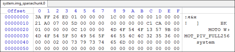
   Fig.8 . sparsechunk_0
   
   It is seen that from the address 0x0000 to the address 0x001B is the header of the sparse file. Further, from the address 0x001C follows the info-group, starting with a piece of type 0xCAC1 , having the length of the data area along with the header 0x100C (address 0x0024 ). Consequently, the next piece will be located starting at the address:
   
   

   0001 + 0100 = 01028 

   
   Let's see what is located at this address: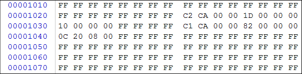
   
   
   Fig.9 . Piece 2
   
   Address 0x1028 is a piece of type 0xCAC2 , having a length of 0x0010 (address 0x1030 ). Then (address 0x1038 ) again a piece of type 0xCAC1 , etc.
   
   The last piece of this file is located at 0x0FFFF524 and is of type 0xCAC3 , i.e. This is a piece of type OFFSET_TO_END , having a size of 0x067AD4 . Delete it as useless: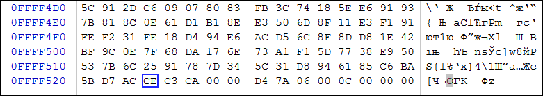
   
   
   Fig.10 . First _sparsechunk_end
   
   So, from the first _sparsechunk file we left only the sparse file header and “data”. Let us also remember the number of pieces that are in the “data” - 0x005D (see the field at 0x0014 ), but this, together with a piece of the OFFSET_TO_END type, therefore, in fact, we “got” only
   
   

    0x005D - 00001 = 0005 

   
   
2. Open the following _sparsechunk file - system.img_sparsechunk.1 in the hex editor:
   
   
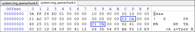
   Fig.11a. The beginning of the second piece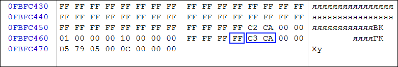
   
   
   Fig.11b. The end of the second piece
   
   Copy the content, discarding the header, the initial and last pieces of type 0xCAC3 , ie, starting from address 0x0028 to address 0xFBFC46C , and add it to the end of the previous part to the place of the remote last piece of type 0xCAC3 (address 0xFFFF524 ). This picture should turn out like this: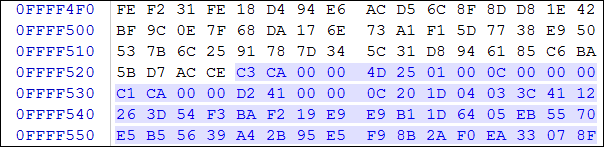
   
   
   Fig.12 . Addition of two parts
   
   Those. we got this "pie":
   
   
   • sparse file header;
   • "Data" of the first _sparsechunk file;
   • "Data" of the second _sparsechunk file.
   
   
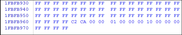
   Fig.13 . End of the folded file
   
   Do not forget to sum up the total number of pieces, i.e. add the number of pieces in the added “data”
   
   

    0x005 + (0x0050 - 00002) = 0x00A 

   
   
3. We continue to perform steps 2 for all the remaining _sparsechunk files except the last. After processing each new file, our “pie” will grow due to the addition of the “data” itself:
   
   
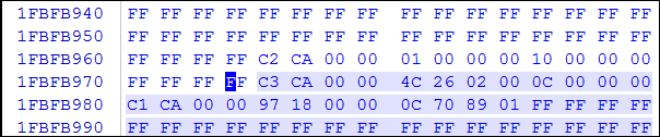
   Fig.14 . Adding a second file
   
   And we continue to summarize the number of pieces ...
4. Add to the "cake" the last _sparsechunk file, following the steps in step 2, discarding only the title and the initial piece of type 0xCAC3 from it . Here's what we got:
   
   
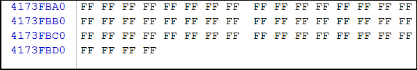
   Fig.15 . Result
   
   The size of this file is 0x4173FBD4 ( 1098120148 or approximately 1047MB), and the total number of pieces is 0x01FB ( 507 ), we write it at 0x0014 (the number of pieces header Total_Chunks field ). 8 pieces that we took away from the total number are pieces of type 0xCAC3: 1 is the final piece from part 0 of the _sparsechunk file, 2 pieces from parts 1-3 and 1 piece from the last (fourth) part.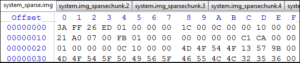
   
   
   Fig.16 . Record the total number of pieces in all _sparsechunk files
   
   If necessary, in the Image_Checksum field (address 0x0018) of the header, enter the checksum calculated using the Crc32 algorithm for the entire file, i.e. header + all pieces. Usually this field is not filled and remains zero.
5. Save the resulting sparse file under the name, for example, system.sparse .

All assembly sparse files from the pieces is completed.

3.2.2.2. Converting a sparse file into a set of _sparsechunk files or cutting (splitting) into chunks

Now let's try to cut the created sparse file into _sparsechunk files. We take 256MB (0x10000000) as the border value.

1. Open the file system.sparse , in which we will perform all the actions described below, in the hex editor:
   
   
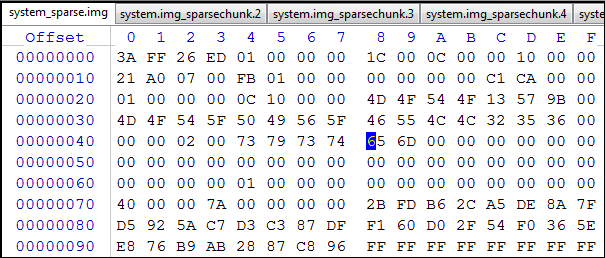
   Fig.17 . system.sparse file
   
   and divide it into separate _sparsechunk parts , containing only “data”.
2. Create the first _sparsechunk file. To do this, go to the offset 0x10000000 from the current position of the marker (for the first file it is 0x0000), i.e. let's get to the maximum size of the future _sparsechunk file. For the first file it will be the address 0x10000000:
   
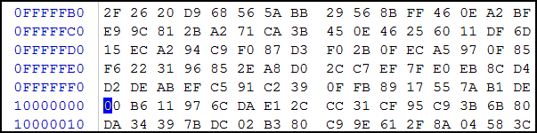
   Fig.18 . _Sparsechunk file boundary
   
   and start looking down the beginning of a piece of any type, i.e. codes 0xCAC1 or 0xCAC2. The nearest piece of type 0xCAC1 is located at 0xFFFF524: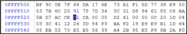
   
   Fig.19 . The boundary of the section _sparsechunk files
   
   To make sure that we have found the most recent piece that “fit” to the dimensions of the “border”, add to the offset found the size of this piece + the size of the header to find the beginning of the next piece:
   
   

    0xFFFF524 + 0x41D2000 + 0x000C = 0x141D1530 

   
   Since displacement of the next piece goes "border", then we found the point of the section _sparsechunk files. Save the code of the system.sparse file from 0x00000000 to 0xFFFF524 to a file, for example, system_new_sparsechunk_0.img .
3. Repeat step 2, taking the beginning of the last piece found in the previous step, i.e. 0xFFFF524 . Let's move the offset 0x10000000 from the current position:
   
   
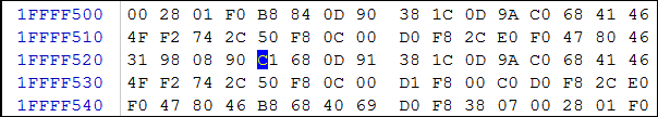
   Fig.20 . The border of the second file
   
   We get the maximum value, i.e. the address of the beginning of the next _sparsechunk part 0x1FFFF524 . Find the nearest piece to the lower side, i.e. Estimated boundary between parts of _sparsechunk files: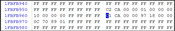
   
   
   Fig.21 . The second boundary of the _sparsechunk files section
   
   Check if we found the last piece correctly, i.e. determine the offset to the next piece:
   
   

    0x1FBFB968 + 0x01897000 + 0x000C = 0x21492968 

   
   Since the offset moves the expected offset of the beginning of the next part, then we correctly found the point of the section _sparsechunk -parts. Save the following code for the system.sparse file from 0xFFFF524 to 0x1FBFB968 to a file, for example, system_new_sparsechunk_1.img .
4. Repeat step 3 to the end of the system.sparse file. As a result, we got a set of the following files:
   
   

     =========================================================================== | № |  |  |  |  | | / |  |  |  |  |  | |=====|===================|========|============|============|==============| | 1 | new_sparsechunk_0 | 256 | 0x00000000 | 0x0FFFF523 | 0x005C ( 92) | | 2 | new_sparsechunk_1 | 252 | 0x0FFFF524 | 0x1FBFB967 | 0x004E ( 78) | | 3 | new_sparsechunk_2 | 242 | 0x1FBFB968 | 0x2EE61403 | 0x00C2 (194) | | 4 | new_sparsechunk_3 | 235 | 0x2EE61404 | 0x3D92DA5B | 0x0074 (116) | | 5 | new_sparsechunk_4 | 62 | 0x3D92DA5C | 0x4173FBD3 | 0x001B ( 27) | |============================================================|==============| | : | 0x01FB (507) | =========================================================================== 

5. Create in each _sparsechunk parts , except the first, because He was there immediately, the title of the sparse file. To do this, copy the header from system.sparse and paste it into each part at the beginning of the file. Using the data from the previous table, we enter the value from the " Number of pieces " column in the Total_Chunks field at 0x0014 of each file.

That's it, the process of cutting into _sparsechunk is complete.

PS All these "horrors" with transitions on shift, search of the necessary pieces, calculation of the sizes of files, etc. I described only in order to show the developer of the MU the procedure necessary to perform work on the processing of sparse - and _sparsechunk files. I never do it myself, because there are computers ... and applications written by me.

Those who wish, having studied the above materials, can themselves create applications to their own taste and color.

4. Creating Dat Files

Dat file is the next step of image compression of partitions. Unlike a sparse file, it contains only informational parts. And to ensure the assembly of the source file, a file called transfer_list is created .

In this case, the source file is divided into parts containing useful information, i.e. info-blocks, and “empty” blocks, i.e. containing zeros. Then all the parts with information are copied in succession to the output file, called new_data , and information about their placement in the source file and the size of these parts is recorded in the transfer_list file.

Thus, the final file with information ( new_data ) does not contain blocks with zeros, i.e. "Shrinks", becoming much smaller in size than the original.

The possibilities of such data conversion and, accordingly, the format of the file transfer_list over time have undergone some changes. There are several versions of this file.

Initially, the new_data file contained all the info blocks, and the transfer_list entered information necessary only for “unclamping”, i.e. to restore full source file. It was version 1, which is used to compress files in the Android OS, starting with version 5.0.0.

Then, besides simple compression, the ability to create patch files to replace only certain parts of the source file, such as a patch for recovery, was added to the dat and transfer_list files, so version 2, used in Android OS starting from version 5.1.0, appeared. This led to even greater compression of the original images, because In general, only changes are transmitted in the patch.

In Android OS 6.0, the approach to the security system has changed a lot, encryption is widely used, respectively, version 3 of the transfer_list file has appeared, allowing you to perform decryption on the fly using stash commands.

4.1.Structure of dat-files

The image of a RAW-format file (.img) after conversion to dat-files (.dat) is a set of the following files:

• transfer_list file This file contains the description of the location of the information parts and the command for their restoration and verification;
• new_data file It contains only the information parts of the source file that are continuously located in it, i.e. no gaps or alignments;
• patch_data file This file contains only parts that replace the information parts of the source file that are continuously located in it, i.e. without gaps or alignments.

Depending on the type of conversion performed on the source file of the RAW format, the composition of the file set may change, but the transfer_list file must always be present, whereas the new_data file and the patch_data file can be either together or separately.

If the conversion consisted in the simple removal of “empty” blocks, then in addition to the transfer_list file, only a new_data file is included in the set, for example, [7] .

If the conversion involved applying the patch, i.e. replacing parts of blocks with others, then only a patch_data file will be present in the set, for example, [8] .

If the conversion consisted of both removing the “empty” blocks, and applying the patch, i.e. replacing parts of the blocks with others, then the new_data file and the patch_data file will be present in the set, for example, [6] .

Consider the structure of each of the dat- files in more detail and begin with the transfer_list file, always used, because namely, it describes the transformations performed on the source file and, accordingly, the actions that must be performed to "get" the source file. I did not say “recovery” because strictly speaking, the source file subjected to conversion may not coincide with the final one obtained after processing. This can occur, for example, after applying a patch, i.e. making changes to the source file.

4.1.1. Structure of the transfer_list file

The file transfer_list is a set of lines of more than 4, each line describes one data field, and has the following structure:

  ==================================================== | № | | | | / |   |   | | | | | |=====|=================|============================| | 1 | Version |   | | 2 | Size New Data |    new_dat | | 3 | Stash Entries |   stash- | | 4 | Stash Max Block | . stash- | | 5 | Commands |    | ==================================================== 

The Version string field describes the version of the transfer_list file and can take values ​​from 1 to 3. File versions differ in their capabilities, which affects the number of lines in the file itself. Version 1 is used for files created for Android version not higher than 5.0. Version 2 is used starting with Android 5.1.0. Version 3 is used starting with Android 6.0.1.

Version 1 does not contain the values ​​described in lines 3 and 4, but must contain at least 2 commands. Therefore, the length of the transfer_list file is at least 4 lines:

• Version ;
• Size New Data ;
• Command 1 ;
• Command 2 .

Versions 2 and 3 can already execute stash commands, so the transfer_list file will contain at least 6 lines:

• Version ;
• Size New Data ;
• Stash Entries ;
• Stash Max Block ;
• Command 1 ;
• Command 2 .

The string field Size New Data describes the size in blocks of the output file new_dat , which contains only info-blocks, i.e. the number of blocks of data being moved. The default block size is 4096 bytes.

The Stash Entries string field describes the number of stash table entries containing a set of offsets to parts of the source file simultaneously used by the stash command.

The Stash Max Block string field describes the maximum size of such a stash part of the source file.

The Command line field contains the command that must be executed to get the target file.

Here is an example transfer_list file version 1:

 1 140333 erase 2,0,190108 new 236,0,56,57,164,517,523,3717,21738,21739,32767,32768,32770,32825,32826,33285... 

where the first line indicates the version of the file (1), the second size of the data being moved, i.e. the size of the new.dat file in blocks (140333). The third and fourth lines contain commands ( erase and new ). These lines are truncated, because too long.

And this is what a transfer_list version 2 file looks like:

 2 317984 129 24931 move 2,117767,117787 20 2,128537,128557 move 2,113788,117574 3786 2,124558,128344 imgdiff 0 2187 2,117631,117633 2 2,128401,128403 imgdiff 2187 2210 2,117788,117902 114 2,128558,128672 move 2,117903,121984 4081 2,164515,168596 move 2,117609,117630 21 2,128379,128400 imgdiff 4397 2229 2,117575,117602 27 2,128345,128372 imgdiff 6626 16212 2,117636,117759 123 2,128406,128529 imgdiff 22838 2170 2,117760,117766 6 2,128530,128536 imgdiff 25008 2198 2,117603,117608 5 2,128373,128378 move 2,125336,125341 5 2,129329,129334 ... move 2,383166,383179 13 2,392851,392864 move 2,383475,383496 21 2,393160,393181 erase 70,32770,32929,32931,33443,65535,65536,65538,66050,98303,98304,98306,98465,98467,98979,131071,131072,131074,131586,163839,163840,163842...,589826,622592,622594,655360 

where in the first line again the version number, in the second the size of the data being moved. 3 and 4 lines are 0, i.e. stash - the table is not used. In lines 5 through the last are the commands erase , move and imgdiff . Some lines are truncated because too long.

Let us consider the structure of the new_data file.

4.1.2. Structure of a new_data-file

This file contains only info-blocks of the source img-file code taken from it during processing. They are arranged strictly in order, without spaces, and are used as a data source for the new command.

Let's take a look at the structure of a new_data file with a specific example. The OTA firmware MU A7010-40 [6] incorporates the files system.new.dat and system.transfer.list .

In the last file, the new command occurs three times, in lines 1901, 1945, and 1946. Because the commands are executed strictly sequentially, then the execution of the nerve command new in line 1901

 new 2,226365,226468 

will lead to reading from the new_dat file of the first 103 blocks, starting from the current position of the read pointer, i.e. from 0, and writing to the output file 103 blocks in the range [226365,226468]. In this case, the read pointer of the source will be moved to the address 103. The next command in line 1945

 new 2,294901,294902 

will lead to reading from the new_dat file of the next 1 block, starting from the current position of the read pointer, i.e. with 103, and records in the output file of 1 block in the range [294901,294902]. In this case, the read pointer of the source will be moved to the address 104. Execution of the following command in line 1946

 new 2,294902,294903 

will lead to reading from the new_dat file of the next 1 block, starting from the current position of the read pointer, i.e. with 104, and records in the output file of 1 block in the range [294902,294903]. In this case, the read pointer of the source will be moved to the address 105.

Thus, a new_dat file should contain 105 blocks of jann, respectively, its length should be 105 * 4096 = 430080, which is in reality.

We now turn to the consideration of the structure of the patch_data file.

4.1.3. The structure of the patch_data file

All patch data is combined into one patch_data file in the update package. The data in this file is the source for the bsdiff and imgdiff commands.

4.2. Description of data structures

All structures describe data ranges, with a block value taken as a data unit, i.e. 4096 bytes. The following data description structures exist:

• range set [rangeset]
• slash range set [stash_rangese]
• input data set <...>

Consider their structure in turn.

4.2.1. The structure of the description of the range of info-blocks (set of ranges [rangeset])

The range set [rangeset] is used in the transfer_list file commands to describe the ranges of the info blocks of both the source and destination of the data. Also used in the stash command to describe stash ranges.

A simple data range is described by two values: a pointer to the first and last element of the range, for example, [23,56). In this case, the left border is included in the range, but the right is not. If there are several ranges, then a description of them requires a set of ranges containing one more element - the number of ranges in the set.

Description of the range set, regardless of the version of the transfer_list file, has the following structure:

 [count,posStart1,posEnd1,posStart2,posEnd2,...] , 

Where

• count is the number of offsets in the range set, i.e. numbers in a row of a set of ranges without the first. The number of info-block ranges is equal to half of this value, since each range is described by a pair of values: the beginning and end of the range;
• posStart1 - offset of the beginning of the first range of info-blocks in the final file, in blocks;
• posEnd1 - offset of the last block of the first range of info-blocks in the final file in blocks;
• posStart2 - offset of the beginning of the second range of info-blocks in the final file in blocks;
• posEnd2 - offset of the last block of the second range of info-blocks in the final file in blocks.

As you can see, the set contains an enumeration of data ranges, each consisting of an enumeration start boundary and an end boundary. And the right border is not included in the listing. The length of the range is calculated as follows: length = end - start.

For example, from the above example of transfer_list file, let's see how the range sets in the move command are described:

 move 2,117767,117787 20 2,128537,128557 

Here are two sets of ranges:

• source range: 2,117767,117787. It means that the range contains two offsets, i.e. the line contains two numbers of offsets - 117767 and 117787, describing one data range. Accordingly, count = 2. Next, the offset of the beginning of the range (posStart = 117767) is located, followed by the offset of the end of the range (posEnd = 117787). Accordingly, the range contains 117787 - 117767 = 20 elements, i.e. its length is 20;
• receiver range: 2,128537,128557. Similarly, for the target range: count = 2, posStart = 128537, posEnd = 128557, length - 20 elements.

The fact that both ranges contain the same number of elements is an attribute of the move operation, i.e. 20 source elements will be moved to 20 receiver elements.

4.2.2.Stash-band structure (stash_rangeset)

A stash range is a set of info blocks designed to store data elements in a specific place, i.e. This range has not only a set of elements (from what offset and to what), but also the name or pointer of the repository.

A set of info- stash- range blocks has the following structure:

  number:[range_set], 

Where

• number is the identification number of the stash store, decimal number;
• [range_set] - a set of data ranges.

For example, the command line looks like this:

 stash 10 2,298306,298307 

means that one (2/2) data range has been created, starting with offset 298306 to offset 298307 (not including it), i.e. the size of one element (298307-298306 = 1), and marked as stash-storage with an identification number of 10.

Another example:

 stash 11 2,295927,295960 

means that one (2/2) data range has been created, starting with offset 295927 to offset 295960 (not including it), i.e. 33 elements in size (295960-295927 = 33), and marked as stash storage with identification number 11.

One more example:

 stash 8 6,247114,247116,247150,247155,247156,247156 

means that 3 (6/2) data ranges:

1) from the offset 247114 to the offset 247116 (not including it), i.e. the size of 2 elements (247116-247114 = 2);

2) starting from offset 247150 to offset 247155 (not including it), i.e. the size of 5 elements (247155-247150 = 5);

3) starting from offset 247156 to offset 247156 (not including it), i.e.0 elements in size (247156-247156 = 0), merged and marked together as a stash storage with identification number 8.

4.2.3. The structure of the input data set <...>

For version 1, this set looks like this:

 [src_rangeset] [tgt_rangeset], 

Where

• [src rangeset] - set of ranges of info-blocks of the source file ( new_dat or patch_dat ), i.e. data source;
• [tgt rangeset] - set of ranges of info-blocks of the output file (* .img), i.e. data receiver.

For version 2 and 3 this set can be of the following types:

1. [tgt_rangeset] <src_block_count> [src_rangeset] ;
2. [tgt_rangeset] <src_block_count> [stash_rangeset] ;
3. [tgt_rangeset] <src_range> <src_loc> [stash_rangeset] ;

Where

• [tgt rangeset] - set of ranges of info-blocks of the output file (* .img), i.e. receiver;
• [src rangeset] - set of ranges of info-blocks of the source file, i.e. source;
• [stash_rangeset] - set of ranges of info-blocks of stash -commands;
• <src_block_count> - the number of info-blocks in the range of the source and receiver;
• <src_range> - the number of stash bands;
• <src_loc> -.

4.3. Structure and description of transfer_list-file commands

The transfer_list file uses the following commands:

• bsdiff, imgdiff - apply patch;
• erase - mark specified areas as empty;
• free - clear the stash area . Available in version 2;
• new - fill in the specified areas of the output file with the information from the new_data file;
• move - move info-blocks in specified areas;
• stash - perform moving of specified areas with preliminary processing. Available in version 2;
• zero - fill in the specified areas of the file with zeros.

4.3.1.Commands “erase”, “new”, “zero”

These commands have the following structure:

 name [rangeset], 

Where

• name - the name of the team;
• [rangeset] - a structure that describes a set of ranges of info blocks.

The erase command marks the empty blocks described by the [rangeset] structure . For example, the execution of the command

 erase 70,32770,32929,32931,33443,... 

from [7, transfer_list file, line 2337] will result in clearing 35 sets of blocks of the output file with the numbers [32770,32929], [32931,33443], etc.

The new command records the source info-blocks, i.e. The new_dat file, in the range set, described by the [rangeset] structure of the receiver, i.e. system.img file Info blocks from the source are selected strictly sequentially.

For example, in [7, transfer_list file] command execution in line 1901

 new 2,226365,226468 

will lead to reading from the new_dat file, starting from the current position of the pointer 103 blocks and writing to the output file in the range [226365,226468].

The zero command clears the specified set of output file ranges, i.e. fills it with zeros. For example, the execution of the command

 zero 2,226365,226366 

will cause the receiver unit 226365 to be cleared.

4.3.2. The "move" command

This command simply copies the info blocks from the source file described by the [src_rangeset] structure into the existing set of output file ranges described by the [tgt_rangeset] structure .

The move command has the following structure:

 move <...>, 

where <...> is a set of input data that differs depending on the version of the transfet_list file .

For example, if a command has the following form:

 move 2,117767,117787 20 2,128537,128557 

and this is the command for moving info-blocks ( move ), then two sets of ranges are described here:

• source range : 2,117767,117787.
  Indicates that the range contains two offsets (count = 2), describing one range of data. Next is the offset of the beginning of the range (posStart = 117767) and next is the offset of the end of the range (posEnd = 117787);
• receiver range : 2,128537,128557.
  Similarly for the receiver: count = 2, posStart = 128537, posEnd = 128557.

4.3.3. The "bsdiff" and "imgdiff" commands

These commands read the info blocks of the source file, perform updates, and change the info blocks written to the output file. Commands differ only in the type of transformations applied to the info blocks.

Both teams have the following structure:

 name <patchstart> <patchlen> <...>, 

Where

• name - the name of the team;
• patchstart - offset of the beginning of the patch area in blocks;
• patchlen - the length of the patch area in blocks;
• <...> is a set of input data.

4.3.4. The "stash" command

This command saves info-blocks in the stash-area . It has the following structure:

 stash <stash_id> <src_range>, 

Where

• <stash_id> is the identifier of the stash range;
• <src_range> is a set of ranges of info-blocks of the stash area .

4.3.5. Team "free"

This command clears the stash area . It has the following structure:

 free <>, 

Where
<...> - is a set of input data.

To be continued…

5. Conclusion

All the above material and examples of its use is only a “multiplication table”, and not a guide to action. Nobody, of course, manually applies patches and does not convert system files ... I just described the principles for performing transformations on "sparse" files, the categories of which mainly include files containing filesystem files.

For processing “sparse” files, of course, computer programs are used, which are already a large number. If hands reach, I will write a review of existing conversion tools.

Starting to write a publication, I wanted to bring to the users only the basics, so to speak, exclusively “theory”. Sincemost of the work on the “digging” in the source texts and firmware was done by me in 2013-2014, then in the process of work I had to work a lot: to remember something, to rethink something, and to thoroughly supplement it with the advent of new versions of android. In the next part, I will describe examples of processing “sparse” files.

There was a lot of material, of course, the article needed to be immediately divided into two or three parts for ease of assimilation and preparation. But as it happened, it happened. This is me about the fact that you do not judge strictly, I also may not know something at all, but do not take into account something ... If you have questions or suggestions, you are welcome.

6. Sources of information

1. Sparse_file.
2. Lenovo s90A device firmware
3. sparse_format.h
4. Lenovo Moto Z
five. Victara_Retail_China_XT1085_5.1_LPE23.32-53_CFC.xml.zip - Lenovo Moto X.
6 A7010a40_S111_150825_ROW_TO_A7010a40_S112_150901_ROW_WC15.zip.
7
eight. OTA update recovery.