In previous articles, we looked at the PostgreSQL indexing mechanism , the interface of access methods and the following methods: hash indices , B-trees , GiST , SP-GiST , GIN and RUM . The topic of this article is BRIN indices.

BRIN

General idea

In contrast to the indexes with which we have already met, the idea of ​​BRIN is not to quickly find the necessary lines, but to avoid looking at obviously unnecessary ones. This is always an inaccurate index: it does not contain TIDs of table rows at all.

Simply put, BRIN works well for those columns whose values ​​correlate with their physical location in the table. In other words, if a query without an ORDER BY clause produces column values ​​in almost ascending or descending order (and there are no indices in the column).
')
The access method was created in the framework of the European project on the extremely large Axle analytical databases with an eye on tables of the size of one and tens of terabytes. An important property of BRIN that allows you to create indexes on such tables is the small size and minimal overhead costs of maintenance.

It works as follows. The table is divided into zones (range) the size of several pages (or blocks, which is the same) - hence the name: Block Range Index, BRIN. For each zone, a summary of the data in that zone is stored in the index. As a rule, this is the minimum and maximum values, but sometimes it happens otherwise, as we will see later. If, when executing a query containing a condition on a column, the desired values ​​do not fall within the range, then the entire zone can be safely omitted; if they do, all the lines in all blocks of the zone will have to be viewed and the appropriate ones selected.

It will not be a mistake to consider BRIN not as an index in the usual sense, but as an accelerator of sequential table scanning. You can look at it as an alternative to partitioning, if each zone is considered a separate “virtual” section.
Now consider the index device in more detail.

Device

The first (or rather, zero) in the index is a page with metadata.

With some indent from the metadata are pages with summary information. Each index line contains a summary of any one zone.

And between the metastpage and the summary data there are pages with a reverse zone map (reverse range map, abbreviated revmap). In essence, this is an array of pointers (TIDs) for the corresponding index rows.



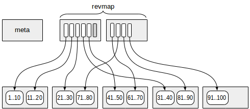
For some zones, the pointer in revmap may not lead to any index line (in the figure it is marked in gray). In this case, it is considered that no summary information is available for this zone.

Index scan

How is an index used if it does not contain references to table rows? Of course, this access method does not know how to return strings one by one, but it can build a bitmap. Bitmap pages are of two types: exact - to the line - and inaccurate - to the page. Inaccurate bitmap is used.

The algorithm is simple. The zone map is sequentially viewed (that is, the zones are sorted in the order of their location in the table). Indexes are used to identify index lines with summary information for each zone. If the zone does not exactly contain the desired value, it is skipped; if it can contain (or if there is no summary information) - all pages of the zone are added to the bitmap. The resulting bitmap is used further as usual.

Index update

More interesting is the case of updating the index when the table changes.

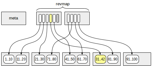
When adding a new version of a row to a table page, we determine which zone it belongs to, and on the zone map we find the index row with summary information. All this is simple arithmetic. Suppose, for example, the zone size is 4 pages, and on page 13 there is a version of the line with the value "42". The zone number (starting from zero) is 13/4 = 3, so in revmap we take, with an offset of 3 (the fourth in a row).

The minimum value for this zone is 31, the maximum is 40. Since the new value of 42 exceeds these limits, we update the maximum value (see figure). If the new value fits into the existing framework, the index does not need to be updated.



All this concerns the case when a new version of the line appears in the zone for which there is already a summary information. When building the index, the summary information is calculated for all existing zones, but with further growth of the table, new pages may appear that fall outside this range. There are two possible options:

1. Usually, an immediate index update does not occur. Nothing wrong with that; as we said, scanning the index will see the entire area. In fact, the update is performed during the cleaning (vacuum), or it can be done manually by calling the function brin_summarize_new_values.
   
2. If you create an index with the autosummarize parameter, the update will take place immediately. But when filling the pages of the zone with new values, the update can be performed very often, so this option is turned off by default.
   

When new zones appear, revmap size may increase. If this card ceases to fit into the pages allotted to it, it simply “captures” the next one, and all versions of the lines that were there are moved to other pages. Thus, the zone map is always located between the metastpage and the summary data.

When you delete a line ... nothing happens. You may notice that in some cases the minimum or maximum value will be removed, and then the range could be reduced. But to determine this, I would have to read all the values ​​in the zone, and this is expensive.

The index correctness does not suffer from this, however, when searching you may need to look at more zones than you really need. In principle, it is possible to manually reassemble the summary information on such a zone (call the functions brin_desummarize_range and brin_summarize_new_values), but how to detect such a need? In any case, there is no standard procedure for this.

Well, updating the line is just removing the old version and adding a new one.

Example

Let's try to build our own mini-data warehouse based on the demo database tables . For example, for the needs of BI-reporting, a denormalized table is needed, reflecting flights departing from the airport or landing at the airport with accuracy to a seat in the cabin. Data for each airport will be added to the table once a day, as soon as it is midnight in the corresponding time zone. Data will not be changed or deleted.

The table will look like this:

demo=# create table flights_bi(
airport_code char(3), --
airport_coord point, --
airport_utc_offset interval, --
flight_no char(6), --
flight_type text. -- : departure () / arrival ()
scheduled_time timestamptz, -- /
actual_time timestamptz, --
aircraft_code char(3), --
seat_no varchar(4), --
fare_conditions varchar(10), --
passenger_id varchar(20), --
passenger_name text --
);
CREATE TABLE

The data loading procedure can be simulated with nested loops: external by days (we take a large database, therefore, 365 days), internal - by time zones (from UTC + 02 to UTC + 12). The request is quite long and does not represent much interest, so I hide it under the spoiler.


demo=# select count(*) from flights_bi;
count
----------
30517076
(1 row)

demo=# select pg_size_pretty(pg_total_relation_size('flights_bi'));
pg_size_pretty
----------------
4127 MB
(1 row)

It turned out 30 million lines and 4 GB. God knows how much, but it’s good for a laptop: I have a full scan in about 10 seconds.

What columns to build the index?

Since BRIN-indexes are small and have low overhead, and updates, if they occur, rarely, there is a rare situation when you can create many “just in case” indexes, for example, across all fields for which analytics users can build your adhoc requests. Not useful - well, and even a not very efficient index will probably work better than a full scan. Of course, there are fields where the index is completely useless; they will be prompted by simple common sense.

But it would be strange to confine to such advice, therefore we will try to formulate a more accurate criterion.

We said that these data should in some way correlate with their physical location. It is appropriate to recall here that PostgreSQL collects statistics on the fields of the tables, which also includes the correlation value. This value is used by the scheduler to choose between conventional index scanning and bitmap scanning, and we can use it to evaluate the suitability of the BRIN index.

In our example, the data is obviously ordered by days (both by scheduled_time and actual_time - the difference is small). This happens because when adding rows to a table (in the absence of deletions and updates), they fit into the file sequentially, one after another. In the load imitation, we did not even use the ORDER BY clause, therefore, within the day, the dates can in principle be mixed as desired, but orderliness must be present. Check:

demo=# analyze flights_bi;
ANALYZE
demo=# select attname, correlation from pg_stats where tablename='flights_bi'
order by correlation desc nulls last;
attname | correlation
--------------------+-------------
scheduled_time | 0.999994
actual_time | 0.999994
fare_conditions | 0.796719
flight_type | 0.495937
airport_utc_offset | 0.438443
aircraft_code | 0.172262
airport_code | 0.0543143
flight_no | 0.0121366
seat_no | 0.00568042
passenger_name | 0.0046387
passenger_id | -0.00281272
airport_coord |
(12 rows)

A value that is not too close to zero (and, ideally, about plus or minus ones, as in our case), suggests that a BRIN index would be appropriate.

The second and third places were unexpectedly the service class fare_condition (the column contains three unique values) and the flight type flight_type (two unique values). This is a snag: formally, the correlation is high, but in fact in several pages taken in succession all the possible values ​​will surely show up - and this means that there will be no sense from BRIN.

Next is the time zone airport_utc_offset: in our example, within a single day cycle, the airports “by construction” are ordered by time zones.

With these two fields - time and time zone - we will continue to experiment.

Possible correlation violation

The correlation “built by construction” can be easily broken by changing the data. And the point here is not to change a particular value, but to a device of multiversion: the old version of the line is deleted on one page, but the new one can be inserted anywhere where there is free space. Because of this, the updates shuffle the lines entirely.

In part, this phenomenon can be dealt with by reducing the value of the storage parameter fillfactor, thereby leaving room on the page for future updates. But do you want to increase the volume of the already huge table? In addition, this does not solve the issue of deletions: they also “prepare traps” for new lines, freeing up space somewhere inside the existing pages. Because of this, lines that would otherwise end up at the end of the file will be inserted in some arbitrary place.

By the way, fun fact. Since there are no references to table rows in the BRIN-index, its presence should not interfere with HOT-updates - but it does.

So, first of all, BRIN is designed for tables of large and even huge size, which are either not updated at all or are updated very little. However, with the addition of new rows (at the end of the table), he handles well. This is not surprising, since this access method was created with an eye to data warehouses and analytical reporting.

What is the size of the zone to choose?

If we are dealing with a terabyte table, then, perhaps, the main concern in choosing the size of the zone will be that the BRIN index does not turn out too large. In our case, we can afford to analyze the data more accurately.

To do this, we can select unique column values ​​and see how many pages these values ​​occur. Localization of values ​​increases the chances of successful use of the BRIN-index. Moreover, the number of pages found will serve as a hint for determining the size of the zone. If the value is “spread” on all pages of the table - BRIN is useless.

Of course, this technique should be applied with a good eye on the internal data structure. For example, it makes no sense for us to consider each date (or rather, the timestamp, which includes time) as a unique value - we need to round it up to days.

A number of technically such an analysis can be performed by looking at the value of the hidden ctid column, which gives a pointer to the row version (TID): the page number and the row number inside the page. Unfortunately, there is no regular way to decompose the TID into its two components, so you have to bring types through a textual representation:

demo=# select min(numblk), round(avg(numblk)) avg, max(numblk)
from (
select count(distinct (ctid::text::point)[0]) numblk
from flights_bi
group by scheduled_time::date
) t;
min | avg | max
------+------+------
1192 | 1500 | 1796
(1 row)

demo=# select relpages from pg_class where relname = 'flights_bi';
relpages
----------
528172
(1 row)

We see that each day is distributed fairly evenly across the pages, and the days are slightly mixed with each other (1500 × 365 = 547500, which is only slightly more than the number of pages in table 528172). This, in fact, is understandable “by construction”.

Valuable information here is a specific number of pages. With a standard zone size of 128 pages, each day will take from 9 to 14 zones. This seems to be adequate: if you request for a particular day, you can expect an error of around 10%.

Let's try:

demo=# create index on flights_bi using brin(scheduled_time);
CREATE INDEX

The size of the index is only 184 KB:

demo=# select pg_size_pretty(pg_total_relation_size('flights_bi_scheduled_time_idx'));
pg_size_pretty
----------------
184 kB
(1 row)

Increasing the size of the zone, sacrificing accuracy, in this case hardly makes sense. And if you wish, you can reduce it - then on the contrary, the accuracy will increase (along with the size of the index).

Now look at the time zones. Here, too, you can not act "in the forehead" - all values ​​should be divided by the number of daily "cycles", since the distribution is repeated within each day. In addition, since there are few time zones, you can view the entire distribution:

demo=# select airport_utc_offset, count(distinct (ctid::text::point)[0])/365 numblk
from flights_bi
group by airport_utc_offset
order by 2;
airport_utc_offset | numblk
--------------------+--------
12:00:00 | 6
06:00:00 | 8
02:00:00 | 10
11:00:00 | 13
08:00:00 | 28
09:00:00 | 29
10:00:00 | 40
04:00:00 | 47
07:00:00 | 110
05:00:00 | 231
03:00:00 | 932
(11 rows)

On average, the data for each time zone is 133 pages per day, but the distribution is very uneven: Petropavlosk-Kamchatsky and Anadyr fit only six pages, and Moscow and the surrounding area require nine hundred. The default zone size is definitely not suitable here; let's set 4 pages for example.

demo=# create index on flights_bi using brin(airport_utc_offset) with (pages_per_range=4);
CREATE INDEX
demo=# select pg_size_pretty(pg_total_relation_size('flights_bi_airport_utc_offset_idx'));
pg_size_pretty
----------------
6528 kB
(1 row)


Execution plan

Now let's see how our indexes work. Choose a day, say, a week ago (“today” is defined in the demo database by the function bookings.now):

demo=# \set d 'bookings.now()::date - interval \'7 days\''
demo=# explain (costs off,analyze)
select *
from flights_bi
where scheduled_time >= :d and scheduled_time < :d + interval '1 day';
QUERY PLAN
--------------------------------------------------------------------------------
Bitmap Heap Scan on flights_bi (actual time=10.282..94.328 rows= 83954 loops=1)
Recheck Cond: ...
Rows Removed by Index Recheck: 12045
Heap Blocks: lossy= 1664
-> Bitmap Index Scan on flights_bi_scheduled_time_idx
(actual time=3.013..3.013 rows= 16640 loops=1)
Index Cond: ...
Planning time: 0.375 ms
Execution time: 97.805 ms


As you can see, the scheduler used the created index. How accurate is it? This is indicated by the ratio of the number of rows that satisfy the conditions of the sample (rows of the Bitmap Heap Scan node) to the total number of rows that was obtained using the index (the same plus Rows Removed by Index Recheck). In our case, 83954 / (83954 + 12045) - approximately 90%, as expected (this value will change from day to day).

Where did the number 16640 appear in the actual rows of the Bitmap Index Scan node? The fact is that this plan node builds an inaccurate (page by page) bitmap and has no idea how many lines it will affect, but it’s necessary to show something. Therefore, because of hopelessness, it is believed that on each page we will find 10 lines. In total, the bitmap contains 1664 pages (this value can be seen from “Heap Blocks: lossy = 1664”) - it turns out to be 16640. In general, this is a meaningless number, you do not need to pay attention to it.

What about airports? For example, let's take Vladivostok time zone, which occupies 28 pages per day:

demo=# explain (costs off,analyze)
select *
from flights_bi
where airport_utc_offset = interval '8 hours';
QUERY PLAN
----------------------------------------------------------------------------------
Bitmap Heap Scan on flights_bi (actual time=75.151..192.210 rows= 587353 loops=1)
Recheck Cond: (airport_utc_offset = '08:00:00'::interval)
Rows Removed by Index Recheck: 191318
Heap Blocks: lossy=13380
-> Bitmap Index Scan on flights_bi_airport_utc_offset_idx
(actual time=74.999..74.999 rows=133800 loops=1)
Index Cond: (airport_utc_offset = '08:00:00'::interval)
Planning time: 0.168 ms
Execution time: 212.278 ms

Again the scheduler uses the BRIN index created. Accuracy is worse (about 75% in this case), but this is expected: the correlation is lower.

Of course, several BRIN indices (like any others) can be combined at the level of a bitmap. For example, data on the selected time zone for the month:

demo=# \set d 'bookings.now()::date - interval \'60 days\''
demo=# explain (costs off,analyze)
select *
from flights_bi
where scheduled_time >= :d and scheduled_time < :d + interval '30 days'
and airport_utc_offset = interval '8 hours';
QUERY PLAN
---------------------------------------------------------------------------------
Bitmap Heap Scan on flights_bi (actual time=62.046..113.849 rows=48154 loops=1)
Recheck Cond: ...
Rows Removed by Index Recheck: 18856
Heap Blocks: lossy=1152
-> BitmapAnd (actual time=61.777..61.777 rows=0 loops=1)
-> Bitmap Index Scan on flights_bi_scheduled_time_idx
(actual time=5.490..5.490 rows=435200 loops=1)
Index Cond: ...
-> Bitmap Index Scan on flights_bi_airport_utc_offset_idx
(actual time=55.068..55.068 rows=133800 loops=1)
Index Cond: ...
Planning time: 0.408 ms
Execution time: 115.475 ms


Comparison with B-tree

What if you build a regular B-tree index on the same field as BRIN?

demo=# create index flights_bi_scheduled_time_btree on flights_bi(scheduled_time);
CREATE INDEX
demo=# select pg_size_pretty(pg_total_relation_size('flights_bi_scheduled_time_btree'));
pg_size_pretty
----------------
654 MB
(1 row)

It turned out several thousand times more than our BRIN! True, the query execution speed slightly increased - the scheduler realized that the data is physically ordered and there is no need to build a bitmap, and, most importantly, do not need to recheck the index condition:

demo=# explain (costs off,analyze)
select *
from flights_bi
where scheduled_time >= :d and scheduled_time < :d + interval '1 day';
QUERY PLAN
----------------------------------------------------------------
Index Scan using flights_bi_scheduled_time_btree on flights_bi
(actual time=0.099..79.416 rows=83954 loops=1)
Index Cond: ...
Planning time: 0.500 ms
Execution time: 85.044 ms

This is the beauty of BRIN: we sacrifice efficiency, but we win a lot of space.

Operator Classes

minmax

For data types whose values ​​can be compared with each other, the summary information consists of the minimum and maximum values. The corresponding operator classes contain minmax in the name, for example, date_minmax_ops. Actually, we have so far considered them, and such are the majority.

inclusive

Comparison operations are not defined for all data types. For example, they are not for points (type of point), which presents the coordinates of airports. By the way, this is why statistics do not show a correlation for this column:

demo=# select attname, correlation
from pg_stats
where tablename='flights_bi' and attname = 'airport_coord';
attname | correlation
---------------+-------------
airport_coord |
(1 row)

But for many of these types, you can introduce the concept of a “bounding area”, for example, a bounding box for geometric shapes. We talked in detail about how this property is used by the GiST index. Similarly, BRIN allows you to collect summary information about columns of these types: the bounding area for all values ​​within a zone is a summary value.

Unlike GiST, the summary value in BRIN must be of the same type as the data being indexed. Therefore, for example, for points an index cannot be built, although it is clear that the coordinates could work in BRIN: the longitude is quite strongly related to the time zone. Fortunately, no one bothers to create an index by expression, transforming points into degenerate rectangles. At the same time, we set the zone size to one page, just to show the extreme case:

demo=# create index on flights_bi using brin (box(airport_coord)) with (pages_per_range=1);
CREATE INDEX

Even in such an extreme version, the index takes only 30 MB:

demo=# select pg_size_pretty(pg_total_relation_size('flights_bi_box_idx'));
pg_size_pretty
----------------
30 MB
(1 row)

Now we can write queries, limiting airports to coordinates. For example:

demo=# select airport_code, airport_name
from airports
where box(coordinates) <@ box '120,40,140,50';
airport_code | airport_name
--------------+-----------------
KHV | -
VVO |
(2 rows)

True, the scheduler will refuse to use our index.

demo=# analyze flights_bi;
ANALYZE
demo=# explain select * from flights_bi
where box(airport_coord) <@ box '120,40,140,50';
QUERY PLAN
---------------------------------------------------------------------
Seq Scan on flights_bi (cost=0.00..985928.14 rows=30517 width=111)
Filter: (box(airport_coord) <@ '(140,50),(120,40)'::box)

Why? Let's disable full scans and see.

demo=# set enable_seqscan = off;
SET
demo=# explain select * from flights_bi
where box(airport_coord) <@ box '120,40,140,50';
QUERY PLAN
--------------------------------------------------------------------------------
Bitmap Heap Scan on flights_bi (cost=14079.67..1000007.81 rows=30517 width=111)
Recheck Cond: (box(airport_coord) <@ '(140,50),(120,40)'::box)
-> Bitmap Index Scan on flights_bi_box_idx
(cost=0.00..14072.04 rows= 30517076 width=0)
Index Cond: (box(airport_coord) <@ '(140,50),(120,40)'::box)

It turns out that the index can be used, but the scheduler believes that the bitmap will have to be built all over the table - no wonder that in this case he prefers a full scan. The problem here is that for geometry types, PostgreSQL does not collect any statistics, so the scheduler has to act blindly:

demo=# select * from pg_stats where tablename = 'flights_bi_box_idx' \gx
-[ RECORD 1 ]----------+-------------------
schemaname | bookings
tablename | flights_bi_box_idx
attname | box
inherited | f
null_frac | 0
avg_width | 32
n_distinct | 0
most_common_vals |
most_common_freqs |
histogram_bounds |
correlation |
most_common_elems |
most_common_elem_freqs |
elem_count_histogram |

Alas. But there are no complaints about the index itself, it works, and not bad:

demo=# explain (costs off,analyze)
select * from flights_bi where box(airport_coord) <@ box '120,40,140,50';
QUERY PLAN
----------------------------------------------------------------------------------
Bitmap Heap Scan on flights_bi (actual time=158.142..315.445 rows= 781790 loops=1)
Recheck Cond: (box(airport_coord) <@ '(140,50),(120,40)'::box)
Rows Removed by Index Recheck: 70726
Heap Blocks: lossy=14772
-> Bitmap Index Scan on flights_bi_box_idx
(actual time=158.083..158.083 rows=147720 loops=1)
Index Cond: (box(airport_coord) <@ '(140,50),(120,40)'::box)
Planning time: 0.137 ms
Execution time: 340.593 ms

The conclusion, apparently, is this: if you need at least something non-trivial from geometry, you need PostGIS. In any case, he is able to collect statistics.

Inside

A peek inside the BRIN-index allows regular extension pageinspect.

First, the meta-information will tell us the size of the zone and how many pages are allocated for revmap:

demo=# select * from brin_metapage_info(get_raw_page('flights_bi_scheduled_time_idx',0));
magic | version | pagesperrange | lastrevmappage
------------+---------+---------------+----------------
0xA8109CFA | 1 | 128 | 3
(1 row)

Here pages 1 through 3 are revmap, the rest is summary data. You can get from revmap links to the summary data for each zone. Say, information about the first zone, covering the first 128 pages of the table, is here:

demo=# select * from brin_revmap_data(get_raw_page('flights_bi_scheduled_time_idx',1)) limit 1;
pages
---------
(6,197)
(1 row)

But the summary data itself:

demo=# select allnulls, hasnulls, value
from brin_page_items(get_raw_page('flights_bi_scheduled_time_idx', 6 ), 'flights_bi_scheduled_time_idx')
where itemoffset = 197 ;
allnulls | hasnulls | value
----------+----------+----------------------------------------------------
f | f | {2016-08-15 02:45:00+03 .. 2016-08-15 17:15:00+03}
(1 row)

Next zone:

demo=# select * from brin_revmap_data(get_raw_page('flights_bi_scheduled_time_idx',1)) offset 1 limit 1;
pages
---------
(6,198)
(1 row)

demo=# select allnulls, hasnulls, value from brin_page_items(get_raw_page('flights_bi_scheduled_time_idx', 6 ), 'flights_bi_scheduled_time_idx') where itemoffset = 198 ;
allnulls | hasnulls | value
----------+----------+----------------------------------------------------
f | f | {2016-08-15 06:00:00+03 .. 2016-08-15 18:55:00+03}
(1 row)

And so on.

For inclusion classes, the value field will display something like

{(94.4005966186523,69.3110961914062),(77.6600036621,51.6693992614746) .. f .. f}

The first value is the enclosing rectangle, and the letters “f” at the end mean the absence of empty elements (the first) and the absence of values ​​that cannot be combined (the second). Actually, the only case of non-joining values ​​is IPv4 and IPv6 addresses (inet data type).

Properties

Let me remind you that the relevant requests were cited earlier .

Method properties:

amname | name | pg_indexam_has_property
--------+---------------+-------------------------
brin | can_order | f
brin | can_unique | f
brin | can_multi_col | t
brin | can_exclude | f

Indexes can be created in multiple columns. In this case, each column collects its own summary information, but for each zone it is stored together. Of course, such an index makes sense if the same zone size is suitable for all columns.

Index properties:

name | pg_index_has_property
---------------+-----------------------
clusterable | f
index_scan | f
bitmap_scan | t
backward_scan | f

Obviously, only bitmap scanning is supported.

But the lack of clustering can cause confusion. It would seem that since the BRIN-index is sensitive to the physical order of rows, then it would be logical to be able to cluster data on it? But no, unless you can create a “regular” index (B-tree or GiST, depending on the type of data) and cluster on it. And by the way, would you like to cluster a supposedly huge table, considering the exclusive lock, operation time and disk space consumption during the rebuild?

Column level properties:

name | pg_index_column_has_property
--------------------+------------------------------
asc | f
desc | f
nulls_first | f
nulls_last | f
orderable | f
distance_orderable | f
returnable | f
search_array | f
search_nulls | t

There are solid dashes, except for the possibility of working with uncertain values.

Ending