Clustering and visualization of textual information
In the Russian-speaking sector of the Internet there are very few educational practical examples (and with an example of a code even less) analysis of text messages in Russian. Therefore, I decided to collect the data together and consider an example of clustering, since data preparation for training is not required.
Most of the libraries used are already in the Anaconda 3 distribution, so I advise you to use it. Missing modules / libraries can be installed as standard via pip install “package name”.
We connect the following libraries:
For analysis, you can take any data. This task came to my eyes then: Statistics of search requests of the project State expenses . They needed to break the data into three groups: private, public, and commercial organizations. I did not want to invent an extraordinary thing, so I decided to check how clustering would lead in this case (looking ahead - not very much). But you can download the data from VK of any public:
I will use search query data to show how short text data clusters poorly. I cleared the special characters and punctuation marks from the text plus the replacement of abbreviations (for example, the individual entrepreneur is an individual entrepreneur). It turned out the text, where in each line there was one search query.
')
We read the data into an array and proceed to normalization - bringing the word to the initial form. This can be done in several ways using Porter Stemmer, MyStem Stemmer and PyMorphy2. I want to warn - MyStem works through the wrapper, so the speed of operations is very slow. Let us dwell on Porter's template, although no one bothers to use others and combine them with each other (for example, go through PyMorphy2, and after Porter's template).
Create a weight matrix TF-IDF. We will take each search query for a document (as they do when analyzing posts on Twitter, where each tweet is a document). We will take tfidf_vectorizer from the sklearn package, and we will take the stop words from the ntlk package (we’ll initially need to download via nltk.download ()). Parameters can be adjusted as you see fit - from the upper and lower bounds to the number of n-gram (in this case, take 3).
Over the resulting matrix, we begin to apply various clustering methods:
The data obtained can be grouped in the dataframe and count the number of queries that fell into each cluster.
Due to the large number of queries, it is not quite convenient to look at the tables and I would like more interactivity to understand. Therefore, we will make graphs of the relative positions of requests relative to each other
First you need to calculate the distance between the vectors. The cosine distance will be used for this. The articles propose to use subtraction from one so that there are no negative values and are in the range from 0 to 1, so we will do the same:
Since the graphics will be two-, three-dimensional, and the original distance matrix is n-dimensional, you will have to apply algorithms for reducing the dimension. There are many algorithms to choose from (MDS, PCA, t-SNE), but we’ll stop the choice on Incremental PCA. This choice was made as a result of practical application - I tried MDS and PCA, but I did not have enough RAM (8 gigabytes) and when I began to use the swap file, I could immediately take my computer to restart.
The Incremental PCA algorithm is used as a replacement for the principal component method (PCA) when the data set to be decomposed is too large to fit in RAM. IPCA creates a low-level approximation for the input data using memory that does not depend on the number of input data samples.
Let's proceed directly to the visualization itself:
If you uncomment the line with the addition of titles, it will look something like this:
Not exactly what one would expect. We use mpld3 to convert the image to an interactive graph.
Now, when you hover on any point in the chart, the text pops up with the corresponding search query. An example of the finished html file can be found here: Mini K-Means
If you want in 3D and with a variable scale, then there is a service Plotly , which has a plugin for Python.
The results can be seen here: Example
And the final point is to perform hierarchical (agglomerative) clustering by the Ward method for creating a dendogram.
findings
Unfortunately, in the field of natural language research there are a lot of unresolved issues and not all data can be easily and easily grouped into specific groups. But I hope that this guide will increase interest in this topic and provide a basis for further experiments.
Most of the libraries used are already in the Anaconda 3 distribution, so I advise you to use it. Missing modules / libraries can be installed as standard via pip install “package name”.
We connect the following libraries:
import numpy as np import pandas as pd import nltk import re import os import codecs from sklearn import feature_extraction import mpld3 import matplotlib.pyplot as plt import matplotlib as mpl For analysis, you can take any data. This task came to my eyes then: Statistics of search requests of the project State expenses . They needed to break the data into three groups: private, public, and commercial organizations. I did not want to invent an extraordinary thing, so I decided to check how clustering would lead in this case (looking ahead - not very much). But you can download the data from VK of any public:
import vk # id session = vk.Session(access_token='') # URL access_token, tvoi_id id : # https://oauth.vk.com/authorize?client_id=tvoi_id&scope=friends,pages,groups,offline&redirect_uri=https://oauth.vk.com/blank.html&display=page&v=5.21&response_type=token api = vk.API(session) poss=[] id_pab=-59229916 #id , id info=api.wall.get(owner_id=id_pab, offset=0, count=1) kolvo = (info[0]//100)+1 shag=100 sdvig=0 h=0 import time while h<kolvo: if(h>70): print(h) # , pubpost=api.wall.get(owner_id=id_pab, offset=sdvig, count=100) i=1 while i < len(pubpost): b=pubpost[i]['text'] poss.append(b) i=i+1 h=h+1 sdvig=sdvig+shag time.sleep(1) len(poss) import io with io.open("public.txt", 'w', encoding='utf-8', errors='ignore') as file: for line in poss: file.write("%s\n" % line) file.close() titles = open('public.txt', encoding='utf-8', errors='ignore').read().split('\n') print(str(len(titles)) + ' ') import re posti=[] # for line in titles: chis = re.sub(r'(\<(/?[^>]+)>)', ' ', line) #chis = re.sub() chis = re.sub('[^-- ]', '', chis) posti.append(chis) I will use search query data to show how short text data clusters poorly. I cleared the special characters and punctuation marks from the text plus the replacement of abbreviations (for example, the individual entrepreneur is an individual entrepreneur). It turned out the text, where in each line there was one search query.
')
We read the data into an array and proceed to normalization - bringing the word to the initial form. This can be done in several ways using Porter Stemmer, MyStem Stemmer and PyMorphy2. I want to warn - MyStem works through the wrapper, so the speed of operations is very slow. Let us dwell on Porter's template, although no one bothers to use others and combine them with each other (for example, go through PyMorphy2, and after Porter's template).
titles = open('material4.csv', 'r', encoding='utf-8', errors='ignore').read().split('\n') print(str(len(titles)) + ' ') from nltk.stem.snowball import SnowballStemmer stemmer = SnowballStemmer("russian") def token_and_stem(text): tokens = [word for sent in nltk.sent_tokenize(text) for word in nltk.word_tokenize(sent)] filtered_tokens = [] for token in tokens: if re.search('[--]', token): filtered_tokens.append(token) stems = [stemmer.stem(t) for t in filtered_tokens] return stems def token_only(text): tokens = [word.lower() for sent in nltk.sent_tokenize(text) for word in nltk.word_tokenize(sent)] filtered_tokens = [] for token in tokens: if re.search('[--]', token): filtered_tokens.append(token) return filtered_tokens # () totalvocab_stem = [] totalvocab_token = [] for i in titles: allwords_stemmed = token_and_stem(i) #print(allwords_stemmed) totalvocab_stem.extend(allwords_stemmed) allwords_tokenized = token_only(i) totalvocab_token.extend(allwords_tokenized) Pymorphy2
import pymorphy2 morph = pymorphy2.MorphAnalyzer() G=[] for i in titles: h=i.split(' ') #print(h) s='' for k in h: #print(k) p = morph.parse(k)[0].normal_form #print(p) s+=' ' s += p #print(s) #G.append(p) #print(s) G.append(s) pymof = open('pymof_pod.txt', 'w', encoding='utf-8', errors='ignore') pymofcsv = open('pymofcsv_pod.csv', 'w', encoding='utf-8', errors='ignore') for item in G: pymof.write("%s\n" % item) pymofcsv.write("%s\n" % item) pymof.close() pymofcsv.close() pymystem3
Executable analyzer files for the current operating system will be automatically downloaded and installed when you first use the library.
from pymystem3 import Mystem m = Mystem() A = [] for i in titles: #print(i) lemmas = m.lemmatize(i) A.append(lemmas) # "" import pickle with open("mystem.pkl", 'wb') as handle: pickle.dump(A, handle) Create a weight matrix TF-IDF. We will take each search query for a document (as they do when analyzing posts on Twitter, where each tweet is a document). We will take tfidf_vectorizer from the sklearn package, and we will take the stop words from the ntlk package (we’ll initially need to download via nltk.download ()). Parameters can be adjusted as you see fit - from the upper and lower bounds to the number of n-gram (in this case, take 3).
stopwords = nltk.corpus.stopwords.words('russian') # - stopwords.extend(['', '', '', '', '', '', '', '', '']) from sklearn.feature_extraction.text import TfidfVectorizer, CountVectorizer n_featur=200000 tfidf_vectorizer = TfidfVectorizer(max_df=0.8, max_features=10000, min_df=0.01, stop_words=stopwords, use_idf=True, tokenizer=token_and_stem, ngram_range=(1,3)) get_ipython().magic('time tfidf_matrix = tfidf_vectorizer.fit_transform(titles)') print(tfidf_matrix.shape) Over the resulting matrix, we begin to apply various clustering methods:
num_clusters = 5 # - - KMeans from sklearn.cluster import KMeans km = KMeans(n_clusters=num_clusters) get_ipython().magic('time km.fit(tfidf_matrix)') idx = km.fit(tfidf_matrix) clusters = km.labels_.tolist() print(clusters) print (km.labels_) # MiniBatchKMeans from sklearn.cluster import MiniBatchKMeans mbk = MiniBatchKMeans(init='random', n_clusters=num_clusters) #(init='k-means++', 'random' or an ndarray) mbk.fit_transform(tfidf_matrix) %time mbk.fit(tfidf_matrix) miniclusters = mbk.labels_.tolist() print (mbk.labels_) # DBSCAN from sklearn.cluster import DBSCAN get_ipython().magic('time db = DBSCAN(eps=0.3, min_samples=10).fit(tfidf_matrix)') labels = db.labels_ labels.shape print(labels) # from sklearn.cluster import AgglomerativeClustering agglo1 = AgglomerativeClustering(n_clusters=num_clusters, affinity='euclidean') #affinity : cosine, l1, l2, manhattan get_ipython().magic('time answer = agglo1.fit_predict(tfidf_matrix.toarray())') answer.shape The data obtained can be grouped in the dataframe and count the number of queries that fell into each cluster.
#k-means clusterkm = km.labels_.tolist() #minikmeans clustermbk = mbk.labels_.tolist() #dbscan clusters3 = labels #agglo #clusters4 = answer.tolist() frame = pd.DataFrame(titles, index = [clusterkm]) #k-means out = { 'title': titles, 'cluster': clusterkm } frame1 = pd.DataFrame(out, index = [clusterkm], columns = ['title', 'cluster']) #mini out = { 'title': titles, 'cluster': clustermbk } frame_minik = pd.DataFrame(out, index = [clustermbk], columns = ['title', 'cluster']) frame1['cluster'].value_counts() frame_minik['cluster'].value_counts() Due to the large number of queries, it is not quite convenient to look at the tables and I would like more interactivity to understand. Therefore, we will make graphs of the relative positions of requests relative to each other
First you need to calculate the distance between the vectors. The cosine distance will be used for this. The articles propose to use subtraction from one so that there are no negative values and are in the range from 0 to 1, so we will do the same:
from sklearn.metrics.pairwise import cosine_similarity dist = 1 - cosine_similarity(tfidf_matrix) dist.shape Since the graphics will be two-, three-dimensional, and the original distance matrix is n-dimensional, you will have to apply algorithms for reducing the dimension. There are many algorithms to choose from (MDS, PCA, t-SNE), but we’ll stop the choice on Incremental PCA. This choice was made as a result of practical application - I tried MDS and PCA, but I did not have enough RAM (8 gigabytes) and when I began to use the swap file, I could immediately take my computer to restart.
The Incremental PCA algorithm is used as a replacement for the principal component method (PCA) when the data set to be decomposed is too large to fit in RAM. IPCA creates a low-level approximation for the input data using memory that does not depend on the number of input data samples.
# - PCA from sklearn.decomposition import IncrementalPCA icpa = IncrementalPCA(n_components=2, batch_size=16) get_ipython().magic('time icpa.fit(dist) #demo =') get_ipython().magic('time demo2 = icpa.transform(dist)') xs, ys = demo2[:, 0], demo2[:, 1] # PCA 3D from sklearn.decomposition import IncrementalPCA icpa = IncrementalPCA(n_components=3, batch_size=16) get_ipython().magic('time icpa.fit(dist) #demo =') get_ipython().magic('time ddd = icpa.transform(dist)') xs, ys, zs = ddd[:, 0], ddd[:, 1], ddd[:, 2] # , #from mpl_toolkits.mplot3d import Axes3D #fig = plt.figure() #ax = fig.add_subplot(111, projection='3d') #ax.scatter(xs, ys, zs) #ax.set_xlabel('X') #ax.set_ylabel('Y') #ax.set_zlabel('Z') #plt.show() Let's proceed directly to the visualization itself:
from matplotlib import rc # font = {'family' : 'Verdana'}#, 'weigth': 'normal'} rc('font', **font) # import random def generate_colors(n): color_list = [] for c in range(0,n): r = lambda: random.randint(0,255) color_list.append( '#%02X%02X%02X' % (r(),r(),r()) ) return color_list # cluster_colors = {0: '#ff0000', 1: '#ff0066', 2: '#ff0099', 3: '#ff00cc', 4: '#ff00ff',} # , - 01234 cluster_names = {0: '0', 1: '1', 2: '2', 3: '3', 4: '4',} #matplotlib inline # data frame, ( PCA) + df = pd.DataFrame(dict(x=xs, y=ys, label=clusterkm, title=titles)) # groups = df.groupby('label') fig, ax = plt.subplots(figsize=(72, 36)) #figsize for name, group in groups: ax.plot(group.x, group.y, marker='o', linestyle='', ms=12, label=cluster_names[name], color=cluster_colors[name], mec='none') ax.set_aspect('auto') ax.tick_params( axis= 'x', which='both', bottom='off', top='off', labelbottom='off') ax.tick_params( axis= 'y', which='both', left='off', top='off', labelleft='off') ax.legend(numpoints=1) # 1 # / , #for i in range(len(df)): # ax.text(df.ix[i]['x'], df.ix[i]['y'], df.ix[i]['title'], size=6) # plt.show() plt.close() If you uncomment the line with the addition of titles, it will look something like this:
10 Cluster Example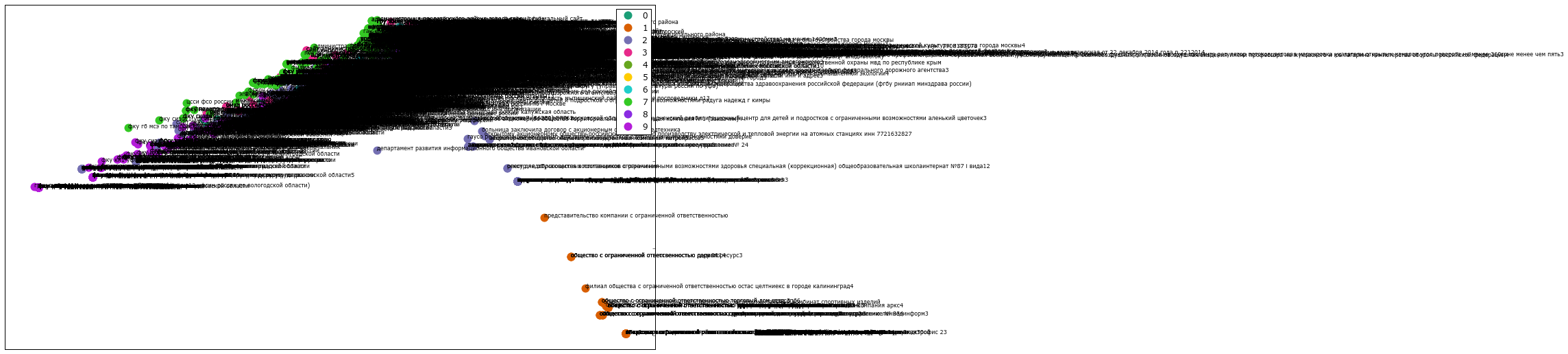
Not exactly what one would expect. We use mpld3 to convert the image to an interactive graph.
# Plot fig, ax = plt.subplots(figsize=(25,27)) ax.margins(0.03) for name, group in groups_mbk: points = ax.plot(group.x, group.y, marker='o', linestyle='', ms=12, #ms=18 label=cluster_names[name], mec='none', color=cluster_colors[name]) ax.set_aspect('auto') labels = [i for i in group.title] tooltip = mpld3.plugins.PointHTMLTooltip(points[0], labels, voffset=10, hoffset=10, #css=css) mpld3.plugins.connect(fig, tooltip) # , TopToolbar() ax.axes.get_xaxis().set_ticks([]) ax.axes.get_yaxis().set_ticks([]) #ax.axes.get_xaxis().set_visible(False) #ax.axes.get_yaxis().set_visible(False) ax.set_title("Mini K-Means", size=20) #groups_mbk ax.legend(numpoints=1) mpld3.disable_notebook() #mpld3.display() mpld3.save_html(fig, "mbk.html") mpld3.show() #mpld3.save_json(fig, "vivod.json") #mpld3.fig_to_html(fig) fig, ax = plt.subplots(figsize=(51,25)) scatter = ax.scatter(np.random.normal(size=N), np.random.normal(size=N), c=np.random.random(size=N), s=1000 * np.random.random(size=N), alpha=0.3, cmap=plt.cm.jet) ax.grid(color='white', linestyle='solid') ax.set_title("", size=20) fig, ax = plt.subplots(figsize=(51,25)) labels = ['point {0}'.format(i + 1) for i in range(N)] tooltip = mpld3.plugins.PointLabelTooltip(scatter, labels=labels) mpld3.plugins.connect(fig, tooltip) mpld3.show()fig, ax = plt.subplots(figsize=(72,36)) for name, group in groups: points = ax.plot(group.x, group.y, marker='o', linestyle='', ms=18, label=cluster_names[name], mec='none', color=cluster_colors[name]) ax.set_aspect('auto') labels = [i for i in group.title] tooltip = mpld3.plugins.PointLabelTooltip(points, labels=labels) mpld3.plugins.connect(fig, tooltip) ax.set_title("K-means", size=20) mpld3.display() Now, when you hover on any point in the chart, the text pops up with the corresponding search query. An example of the finished html file can be found here: Mini K-Means
If you want in 3D and with a variable scale, then there is a service Plotly , which has a plugin for Python.
Plotly 3d
# 3D import plotly plotly.__version__ import plotly.plotly as py import plotly.graph_objs as go trace1 = go.Scatter3d( x=xs, y=ys, z=zs, mode='markers', marker=dict( size=12, line=dict( color='rgba(217, 217, 217, 0.14)', width=0.5 ), opacity=0.8 ) ) data = [trace1] layout = go.Layout( margin=dict( l=0, r=0, b=0, t=0 ) ) fig = go.Figure(data=data, layout=layout) py.iplot(fig, filename='cluster-3d-plot') The results can be seen here: Example
And the final point is to perform hierarchical (agglomerative) clustering by the Ward method for creating a dendogram.
In [44]: from scipy.cluster.hierarchy import ward, dendrogram linkage_matrix = ward(dist) fig, ax = plt.subplots(figsize=(15, 20)) ax = dendrogram(linkage_matrix, orientation="right", labels=titles); plt.tick_params(\ axis= 'x', which='both', bottom='off', top='off', labelbottom='off') plt.tight_layout() # plt.savefig('ward_clusters2.png', dpi=200) findings
Unfortunately, in the field of natural language research there are a lot of unresolved issues and not all data can be easily and easily grouped into specific groups. But I hope that this guide will increase interest in this topic and provide a basis for further experiments.
Source: https://habr.com/ru/post/346206/
All Articles