Attribution using the Markov chain

Business challenge

One of our clients actively used marketing channels of traffic to promote their services and products. After some time, the data on all marketing channels was uploaded to the BigQuery storage, and we decided that it was time to do something interesting with them. For example, expand and modify their analytical modules to optimize marketing costs. In particular, to realize the ability to use more complex attribution of channels using Markov chains, which was not Google Analytics at the time, and perhaps now is not.

We talked in our blog about some common problems of attribution of advertising channels. Here we will discuss only the use of Markov chains.

Markov chains

Markov chains are one of the extremely simple, but elegant tools for studying dynamics in stochastic systems, which is used, among other things, in the attribution of goods. Quite a lot has been written about this, and examples of describing such attribution on the Internet are fairly easy. Our job is to present your attribution method using this tool. But first you need to tell a little about what it is for those who do not know. And who knows, you can safely skip this part.

Let our system be only in a few fixed states. And in each state the probability of transition to any other possible state of this system is strictly and unambiguously determined.

To understand how this happens, you can consider an example of a system that Andrei Andreevich Markov himself (senior) investigated. As a system, he considered the random process of the appearance of a letter in the text. For the basis for the formation of the model, he used the text of “Eugene Onegin”. It is intuitively obvious that the probability of the next letter is largely determined by the previous one. For example, the letter “z” rarely comes after “h”, and the letter “a” is often, and the combination “space” - “s” is generally impossible in a literary language. In general, poor Andrei Andreevich had to count all the letters of this wonderful work of Pushkin in order to understand which letters often follow which ones, because there were no computers at that time.

The only thing that remains is to describe what is happening in the language of mathematics.

Let there be a system with discrete states $$$S = \ lbrace s_1, s_2, ..., s_N \ rbrace$ . Time is set in such a way that at each discrete time step a transition occurs to one of the existing states. Thus, in essence, we exclude from consideration and consider only those iterations in which state jumps occur. Each state is described by a set of conditional probabilities of transition to any state of the system:

$$

$$s_1 = \ lbrace p (s_1 | s_1), p (s_2 | s_1), ... \ rbrace$$

For greater clarity and utility, people tend to write this in the form of a transition probability matrix:

$$

$$M = \ begin {bmatrix} p (s_1 | s_1) & p (s_1 | s_2) & ... \\ p (s_2 | s_1) & p (s_2 | s_2) & ... \\ \ vdots & \ vdots & \ ddots \ end {bmatrix}$$

Or in the form of a transition graph, as in the example from Wikipedia :

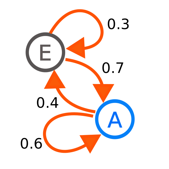
Author: Joxemai4 - Own work, CC BY-SA 3.0, commons.wikimedia.org/w/index.php?curid=10284158

The picture shows a system with two states E and A. The probability of transition from A to A is 0.6, and from A to E is 0.4. It is obvious that the sum of the conditional probabilities of transition from one state should be equal to one. And the sums of each of the lines of the matrix M must also be equal to 1.

But we do not really need conditional probabilities. We need absolute probabilities of the state of the system. And we have the opportunity to learn this, provided that we know what state s0 we started from, ie we have a vector of zeros with a unit in the state in which we are. To do this, we use the full probability formula for the first step of the system:

$$

$$s ^ 1 = s ^ 0 \ times M$$

From this expression, a recurrent formula is obvious, by which one can find the absolute probability at any step of the system, having the distribution from the previous step. Sometimes these distributions converge, sometimes not. For example, for the above example from the picture, the absolute probability of being in E tends to 0.3636 (36), and for A to 0.6363 (63).

But in our problem this is not the case, so it is worthwhile to stop here and go on to the channel attribution itself.

Attribution using the Markov chain

For a start, it's worth telling a little about how the transition probability matrix is ​​compiled.

As each line of “Eugene Onegin” was carefully considered by A. Markov, we consider the chains of channels and fix transitions between channels in the matrix. For example, if we hit the chain from the channel with index 1 into the channel with index 2, then one is added to the matrix element in the first row and second column.

When we walked this way over the entire statistics of the chains, we divide each row of the resulting matrix by the sum of the elements of this row and get those conditional probabilities. And then actually begins the method of attribution.

Let there be $$$N$ attribution channels and calculated transition probability matrix $$$M$ dimensions $$$(N + 1) × (N + 1)$ . $$$(N + 1)$ because, apart from all channels, there is also a transition to the “conversion” state. This is the terminal state, so the last row of the matrix $$$M$ consists of zeros and the last element is 1. In addition, we have a vector $$$L$ - the distribution of lengths of the converted attribution chains for the entire period. Those. if a $$$L_5 = 100,$ This means that the database contains 100 chains containing 5 attribution channels, which end in conversion. In the following, we use:

$$$$ display $$ \ begin {equation} L '(K) = \ lbrack L_1, L_2, ...., L_K \ rbrack / \ sum \ limits_ {k = 1} ^ {K}, L_k \ tag {1 } \ end {equation} $$ display $$

normalized to a certain member $$$K \ le | L |$ distribution.

For each channel $$$i \ in 1,2, ..., N$ It is considered a certain probability indicator to come to a conversion, provided that the chain starts from this channel. Naturally, the word probability here is already used rather conditionally, because it is just some indicator that can be compared with indicators for other channels. This indicator is considered as follows:

Let there be a starting point of a Markov chain, which indicates the channel from which we begin to consider probabilities. This is a vector $$$V_0, | V_0 | = N + 1$ . Vector consists of zeros and only $$$V_i ^ 0 = 1$ . We consider chains of lengths from 1 to $$$K \ le | L |$ . For each chain, the distribution of absolute probabilities is calculated, subject to the beginning of $$$V_0$ .:

$$

$$D_k = D_ {k-1} \ times M, \ tag {2}$$

Where $$$D_k-1$ distribution of absolute probabilities on $$$k-1$ step of the chain, and (×) is the matrix multiplication. It's obvious that $$$D_0 = V_0$ . In the last step, we choose the probability of transition to the terminal $$$p_ {N + 1, k}$ state as a “measure” of the initial channel efficiency. Next, we consider the channel performance indicator using the following formula:

$$

$$E_i = \ sum \ limits_ {k = 1} ^ {K} p_ {N + 1, k} * \ tilde {L} _k, \ tag {3}$$

where (*) is the elementwise multiplication, and $$$\ tilde {L} = L ’(K)$ .

Considering in this way the values ​​of indicators for each of the channels, we obtain comparable performance estimates in the array $$$E$ that can be used for attribution. At attribution, each channel in the chain is assigned a weight of $$$E$ and further weights are normalized. Let there is a chain of channel indexes $$$C$ in which there are no identical adjacent channels and which ends in conversion. Then you can calculate the attribution of channels as follows. Set the vector of zeros $$$W$ dimensions $$$N$ and we will fill it as follows:

$$

$$W_i = \ sum \ limits_ {j = 1} ^ {| C |} \ left \ {\ begin {array} {ll} C_i = 1, if & i = j \\ C_i = 0, if & i \ ne j \ end { array} \ right. \ tag {4}$$

Then the normalized channel attribution vector will be considered as:

$$

$$A = (E * W) / \ sum (E * W) \ tag {5}$$

.

Normalization in this situation is required in order to attribute exactly one conversion. Or, if we consider the conversion through the income that it brought, the income distributed through the channels in the amount should converge, respectively, the formula (5) just appears income multiplier with the conversion.

Example

Suppose there are two channels of attribution with certain transition probabilities, which are given by the transition probabilities matrix:

$$

$$M = \ begin {bmatrix} 0.7 & 0.1 & 0.2 \\ 0.5 & 0.2 & 0.3 \\ 0 & 0 & 1 \ end {bmatrix}, L = \ lbrack 100, 50, 30, 10, 5, 0, .. . \ rbrack$$

We will consider K = 2, then, by the formula (1) $$$L ’(2) = \ lbrack 0.67, 0.33 \ rbrack$ . We calculate the absolute probabilities for chains of length 1 and 2 for the first channel by the formula (2):

$$

$$D_ {1,1} = \ begin {bmatrix} 1 & 0 & 0 \ end {bmatrix} \ times \ begin {bmatrix} 0.7 & 0.1 & 0.2 \\ 0.5 & 0.2 & 0.3 \\ 0 & 0 & 1 \ end {bmatrix} = \ begin {bmatrix} 0.7 & 0.1 & 0.2 \ end {bmatrix}$$

$$

$$D_ {1,2} = \ begin {bmatrix} 0.7 & 0.1 & 0.2 \ end {bmatrix} \ times \ begin {bmatrix} 0.7 & 0.1 & 0.2 \\ 0.5 & 0.2 & 0.3 \\ 0 & 0 & 1 \ end {bmatrix} = \ begin {bmatrix} 0.54 & 0.09 & 0.37 \ end {bmatrix}$$

Then the channel efficiency indicator is calculated as follows using formula (3):

$$

$$E_1 = 0.2 * 0.67 + 0.37 * 0.33 = 0.256$$

We calculate the absolute probabilities for chains of length 1 and 2 for the second channel:

$$

$$D_ {2,1} = \ begin {bmatrix} 0 & 1 & 0 \ end {bmatrix} \ times \ begin {bmatrix} 0.7 & 0.1 & 0.2 \\ 0.5 & 0.2 & 0.3 \\ 0 & 0 & 1 \ end {bmatrix} = \ begin {bmatrix} 0.5 & 0.2 & 0.3 \ end {bmatrix}$$

$$

$$D_ {2,2} = \ begin {bmatrix} 0.5 & 0.2 & 0.3 \ end {bmatrix} \ times \ begin {bmatrix} 0.7 & 0.1 & 0.2 \ 0.5 & 0.2 & 0.3 \\ 0 & 0 & 1 \ end {bmatrix} = \ begin {bmatrix} 0.45 & 0.09 & 0.46 \ end {bmatrix}$$

Then the channel efficiency indicator is calculated as follows:

$$

$$E2 = 0.3 * 0.67 + 0.46 * 0.33 = 0.353$$

Thus, the full vector of channel performance indicators $$$E = [0.256, 0.353] ^ T$ .

Suppose we have a chain of channels $$$C = [1,2,1]$ which ends in conversion. Then by the formula (4):

$$

$$W1 = 1 + 0 + 1 = 2, W2 = 0 + 1 + 0 = 1.$$

And by the formula (5), the attribution of this conversion can be calculated:

$$

$$A = ([0.256, 0.353] T * [2,1]) / (0.256 * 2 + 0.353 * 1) = [0.59, 0.41].$$

Addition

In principle, during attribution, you can use for each channel a weight that corresponds to the transition probability for a chain length equal to the “distance” in the chain from this channel to conversion. Then, for example, in the above example, attribution would be considered as:

$$

$$A = \ frac {[(D_ {1,1} + D_ {1,3}), D_ {2,2}]} {D_ {1,1} + D_ {1,3} + D_ {2, 2}} = \ frac {[(0.2 + 0.51), 0.46]} {0.2 + 0.51 + 0.46} = [0.61,0.39]$$

The same can be done with weights $$$L ’$ which for a chain of length 3 are calculated as $$$L ’(3) = [0.55, 0.28, 0.17]$ . Then the attribution will be as follows:

$$

$$A = \ frac {[(D_ {1,1} \ tilde {L} _1 + D_ {1,3} \ tilde {L} _3), D_ {2,2} \ tilde {L} _2]} { D_ {1,1} \ tilde {L} _1 + D_ {1,3} \ tilde {L} _3 + D_ {2,2} \ tilde {L} _2} = \ frac {[(0.2 \ cdot 0.55+ 0.51 \ cdot 0.17), 0.46 \ cdot 0.28]} {0.2 \ cdot 0.55 + 0.51 \ cdot 0.17 + 0.46 \ cdot 0.28} = [0.6,0.4]$$

Thus, such attribution can be a very useful tool for analyzing traffic, which will allow you to look at it from various sides, even within the framework of one approach. Such methods easily adapt to their goals and are complemented by taking into account known data. For example, the natural next step of “developing” this approach may be adding time to the analysis and taking into account the amount of time between transactions (another intermediate position in the matrix of conditional probabilities, when for some period there were no transitions). All for people, as they say.

This project was completed as part of the work performed by Maxilect, other projects in this category can be found here .