Parallel data sorting in GPU

In this article I will introduce you to the concept of parallel sorting . We will discuss the theory and implementation of a pixel shader.

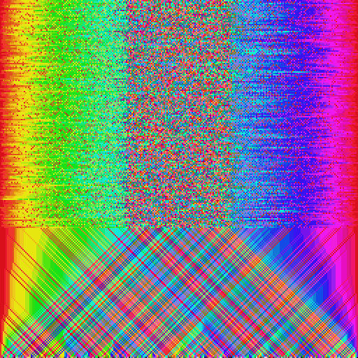
Gif

Introduction

If you studied computer theory in the 80s or 90s, chances are that you tried hard to understand what some developers find delightful in sorting algorithms . What initially seems an insignificant task turns out to be the cornerstone of Computer Science.
')
But what is the "sorting algorithm"? Imagine that you have a list of numbers. The sorting algorithm is a program that gets this list and changes the order of the numbers in it. The concept of sorting algorithms is often introduced in the study of computational complexity - another extensive area of knowledge, which I will discuss in detail in future articles. There are an infinite number of ways to sort the list of items, and each strategy provides its own unique compromise between cost and speed.

Most of the complexity of sorting algorithms arises from how we define the problem, and how we approach its solution. To decide how to reorder elements, the algorithm must compare numbers. Scientifically, each comparison made increases the complexity of the algorithm. Complexity is measured by the number of comparisons performed.

However, not everything is so simple: the number of comparisons and replacement of elements depends on the list itself. That is why in the theory of computers there are more effective ways to evaluate the performance of the algorithm. What is the worst case scenario? What is the maximum number of steps he will take to sort the most unsorted list that he can work with? This way of looking at a problem is known as worst case analysis. We can ask the same question in the best possible scenario. What is the minimum number of comparisons the algorithm must perform to sort the array? If simplified, the latter task often refers to the designation “O” large , which measures complexity as a function of the number of elements to be sorted.

$n$ . It is proved that under such conditions no algorithm can run faster than

$\ mathcal {O} \ left (n \ log n \ right)$ . This means that there can be no algorithm that always sorts any incoming array of length

$n$ by performing less than

$n \ log n$ comparisons.

But O (n log n) means something else!

If you are familiar with the designation “O” large, you can understand that in the previous paragraph we have very simplified the explanation.

One can imagine “O” large as a way of expressing a “ order of magnitude ” function. I.e

$\ mathcal {O} \ left (n \ log n \ right)$ with

$10$ elements doesn't really mean that there will be

$33$ comparisons. There may be 10, or even 100 times more. For a superficial understanding, it is important that the number of comparisons needed to sort an array grows in proportion to

$n \ log n$ .

In future articles I will discuss the topic of computational complexity from a purely mathematical point of view.

Video processor limitations

Traditional sorting algorithms are created based on two main concepts:

Comparison : an operation that compares two list items and determines which one is larger;
Replace : relocation of two items to bring the list closer to the desired state.

The list that needs to be sorted is often specified as an array. Access to arbitrary elements of the array is extremely efficient, and in it without any restrictions you can swap any two elements.

If we want to use a shader for sorting, then we will first have to deal with the inherent limitations of the new environment. Although the list of numbers can be passed to the shader, this will not be the best way to use its parallelism. Conceptually, you can imagine that the GPU executes the same shader code simultaneously for each pixel. Usually this does not happen, because the video processor probably does not have enough computing power to parallelize the calculations for each pixel. Some parts of the image will be processed in parallel, but we should not make assumptions about which parts it is. Therefore, the shader code should be executed under the same restrictions of true parallelism, even if in fact it is not always executed this way.

However, a more serious limitation is that the shader code is localized. If the GPU executes part of the code for a pixel in the coordinate

$\ left [x, y \ right]$ , we cannot write to any other pixel, except

$\ left [x, y \ right]$ . In the shader, the replace operation requires synchronization of both pixels.

Sorting in the video processor

The concept of the approach presented in this article is simple.

Sorted data is transmitted as a texture;
If we have an array $n$ elements, we create texture by size $n \ times 1$ pixels;
The value of the red channel of each pixel contains the number to be sorted;
Each rendering pass will bring the array closer to its final state.

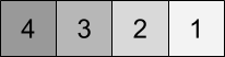
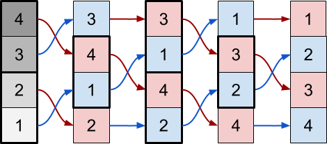
For example, let's imagine that we have to sort a list of four numbers:

$\ left [4,3,2,1 \ right]$ . We can pass it to the shader by creating a texture from

$4 \ times 1$ pixels, keeping the values in the red channel:

As mentioned above, the operation of changing places when executed in a shader is much more complicated, because it must be performed in parallel by two independent pixels. The easiest way to work with such a restriction is to swap adjacent pairs of pixels:

It is important to add that, compared with the execution in the CPU, the process is performed in almost the opposite order. The first pixel samples its previous value.

$4$ and the value on the right

$3$ . Since it is left in the replacement pair , it must accept the smaller of the values. The second pixel must perform the opposite operation.

Since these calculations are performed independently of each other, both parts of the code must "agree" without any communication, which of the values should be dropped down. This is the difficulty of parallel sorting. If we are not careful, both pixels of the replacement pairs will take the same number, thus duplicating it.

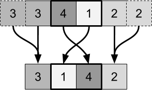
If we repeat the replacement process, nothing will change. Each pair can be sorted in one step. Reproduction of this process will not lead to any changes. To cope with this, you need to change the replacement pairs. We can see this in the following diagram:

What about pixels around the edges?

There are several solutions that can be used to extend this solution to work with the first and last pixels.

The first approach is to consider these two pixels as part of one replacement pair. This approach will work, but will require the creation of additional conditions, which in the shader code will inevitably lead to a decrease in performance.

A simpler solution is to simply trim the texture. The two outermost pixels will perform replacements with themselves:

We can alternately use these two steps until the entire image is sorted:

This technique has existed for quite some time, and is implemented in a variety of styles and variations. Often it is called odd-even sorting , because replacement pairs have odd / even and even / odd indices. This working mechanism is deeply connected with bubble sorting, so it is not surprising that the algorithm is often called parallel bubble sorting .

Complexity

When working with a video processor, we must assume that the same shader code is simultaneously executed for each pixel. In a traditional CPU, we must consider each comparison / replacement as a separate operation. The shader pass will be considered

$n$ operations. If we assume that we can calculate them all in parallel, then the execution time of one and

$n$ will be the same. Therefore, the parallel complexity of each pass of the shader is

$1$ .

What will be the worst case complexity? We see that each step moves a pixel to its final position. Maximum pixel displacement is

$n$ that is, to sort the list we need no more

$n$ steps.

If you look at this task from a more traditional perspective, everything becomes more complicated. Each pass of the shader analyzes each pixel at least once, that is, adds complexity

$n$ . Combined with the number of passes

$n$ it provides complexity

$\ mathcal {O} \ left (n ^ 2 \ right)$ . This shows us how ineffective even-odd sorting is when performing sequentially.

Part 2. Shader implementation.

Shaders for simulation

Shaders are usually used to process the textures they pass. The results of their work are visualized on the screen, and the textures themselves do not change. In this article we want to do something different, because we want the shader to work iteratively with one texture. We discussed in detail how this is done in the previous series of posts How to Use Shaders for Simulations .

The idea is to create two render textures - special textures that can be changed in the shader. The diagram below shows how this process works.

Two render textures are cyclically reversed so that the shader pass uses the previous one as input, and the second as output.

In this article we will use the implementation presented in the post How to Use Shaders for Simulations . If you have not read it yet, then do not worry. We will focus only on the algorithm itself, you just need to know the following:

float4 frag(vertOutput i) : COLOR { //  X, Y  [0, _Pixels-1] float2 xy = (int2)(i.uv * _Pixels); float x = xy.x; float y = xy.y; // UV-  [0,1] float2 uv = xy / _Pixels; // UV-   float s = 1.0 / _Pixels; ... }

The fragmentary function of the shader will contain the sort code. The variable uv denotes the UV coordinates of the current pixel being drawn, and s represents the size of a pixel in UV space.

Reorder in pair replacement

In the previous section, we introduced the concept of a substitution pair . Pixels are grouped into pairs, which are then sorted in a single shader pass. Let's imagine two adjacent pixels whose colors

$x$ and

$y$ represent two numbers. A shader pass must sample these two pixels and change their order accordingly.

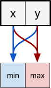
To do this, the pixel from the left side of the replacement pair samples two pixels above and selects as its final color.

$min \ left (x, y \ right)$ . The pixel on the right does the opposite:

The position of a pixel determines not only the operations that need to be done, but also the sampled pixels. Min pixels should sample pixels in the current position and to the right of it. Max pixels should sample the pixel on the left.

 //  max float3 C = tex2D(_MainTex, uv).rgb; //   float3 L = tex2D(_MainTex, uv + fixed2(-s, 0)).rgb; //   result = max(L, C); //  min float3 C = tex2D(_MainTex, uv).rgb; //   float3 R = tex2D(_MainTex, uv + fixed2(+s, 0)).rgb; //  result = max(C, R);

In addition, the min and max pixels are swapped after each operation. The diagram below shows which pixels perform the operation min (blue), and which ones - operation max (red):

The two determining factors in the choice of the operation being performed are the iteration number _Iteration and the index of the element x (or y , if we sort not the rows, but the columns).

Looking at the above scheme, we can derive the last condition, which allows to determine which operation should be performed - min or max:

 //  / #define EVEN(x) (fmod((x),2)==0) #define ODD(x) (fmod((x),2)!=0) float3 C = tex2D(_MainTex, uv).rgb; //  if ( ( EVEN(_Iteration) && EVEN(x) ) || ( ODD (_Iteration) && ODD (x) ) ) { //  max float3 L = tex2D(_MainTex, uv + fixed2(-s, 0)).rgb; //  result = max(L, C); } else { //  min float3 R = tex2D(_MainTex, uv + fixed2(+s, 0)).rgb; //  result = min(C, R); }

This condition ensures that during even iterations (second, fourth, ...) the pixels in the even position will perform the operation max, and the pixels in the odd position will perform the operation min. In the odd iterations (first, third, ...) the opposite happens.

In order for this effect to work, both the render textures need to be set to Clamp , because the shader code has no boundary conditions that prevent access to pixels outside the texture.