Mathematical models of relay-pulse regulators

Introduction
The most important task of automatic control of any technological processes is the development of a mathematical description, calculation and analysis of the dynamics of automatic control systems (ASR).
')
The practice of industrial use of microprocessor control devices (MCI) has shown that “ideal algorithms” are not physically feasible. The ASR synthesized on their basis does not reflect the behavior of the real system [1].
Deviations of algorithms from idealized under certain conditions, for example, for relay-switching regulators, when the speed of the actuator corresponds to the real dynamics of the object, the behavior of the real system with a sufficient degree of accuracy corresponds to the results of the mathematical model.
Relay-pulse controllers are used in microprocessor-based control devices, where the following trend is observed. For example, publication [2] describes the possibilities of using the modbus protocol to create your own Scada system based on Python.
The publication [3] describes the use of Python to work with Arduino. I continue this trend and I hope that Python will finally take over this new area of application.
1. Typical linear control algorithms
I give ideal control algorithms, which are determined by the equations:
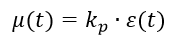
P-algorithm:
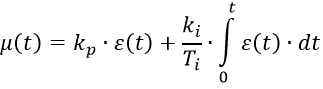
PI algorithm:
PID algorithm:

Where
 - regulatory impact;
  - mismatch signal; Kp, Ki, Kd is the transmission coefficient and Ti, Td are the time constants of the corresponding links (controller settings).
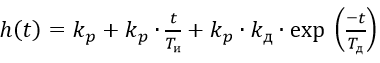
All transitional characteristics of the regulators, taking into account the settings, can be represented by one general formula, avoiding the uncertainty from dividing by 0:
from numpy import e,arange def hp(t,Kp,Ki,Kd,Td): if t<0: z=0 elif Td==0: z=Kp+Ki*t else: z=Kp+Ki*t+Kp*Kd*e**(-t/Td) return z It should be noted that the PID controller is not physically realistic in its ideal form, therefore it is presented in the form of: Kp + Ki * t + Kp * Kd * e ** (- t / Td) to simulate ideality.
Transient characteristics of ideal regulators
#!/usr/bin/env python #coding=utf8 import matplotlib.pyplot as plt import matplotlib as mpl mpl.rcParams['font.family'] = 'fantasy' mpl.rcParams['font.fantasy'] = 'Comic Sans MS, Arial' from numpy import e,arange def hp(t,Kp,Ki,Kd,Td): if t<0: z=0 elif Td==0: z=Kp+Ki*t else: z=Kp+Ki*t+Kp*Kd*e**(-t/Td) return z x=arange(-2,10,0.01) y=[hp(t,2,0,0,0) for t in x] y1=[hp(t,2,0.25,0,0) for t in x] y2=[hp(t,2,0.25,2,2) for t in x] plt.title(' ') plt.plot(x, y, linewidth=2, label=' ') plt.plot(x, y1, linewidth=2, label=' ') plt.plot(x, y2, linewidth=2, label=' ') plt.legend(loc='best') plt.grid(True) plt.show() The nature of the transients is shown in the graph:
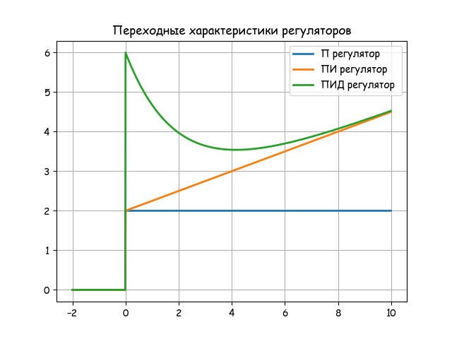
On the basis of typical ideal control algorithms, methods of optimal parametric synthesis are developed in control theory and the general properties of ASR are investigated.
In industrial automatic regulators, typical algorithms are implemented approximately. The deviation of the control algorithm from the ideal does not have a significant effect on the behavior of the system if the controller is operating in the area of “normal” modes.
For this, it is necessary to know and take into account the essential features of the real algorithm, due to the method of its technical implementation. In the practice of automation, electrical (electronic) indirect action regulators in the form of virtual modules of microprocessor controllers are widely used.
Consider the classification of automatic electric regulators according to the method of implementation of the algorithm [1]:
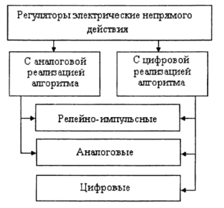
In accordance with the presented classification in this and subsequent publications, the implementation of mathematical models of regulators by means of Python will be considered.
2. Pulse relay controllers
In automatic process control systems, actuators are used with electric asynchronous reversing motors with a constant output rotation speed. This determined the method of implementation of the regulation algorithm.
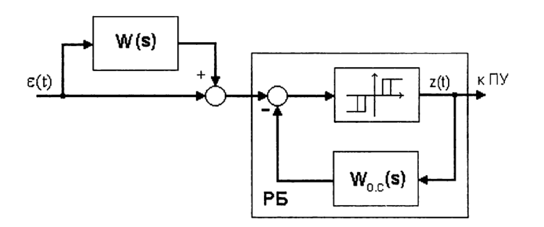
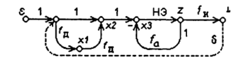
The principle of implementation of the PI algorithm in the presence of constant speed EIM is illustrated by the scheme shown in the figure:
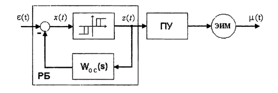
The regulating unit (RB) forms the rectangular impulses of constant amplitude that control the EIM, the duration and duty cycle of which depend on the values of the controller settings and the value of the input signal.
The direct channel of the RB contains a non-linear element - a three-position relay with a dead zone ∆n a ∆v return zone, shown in the figure:
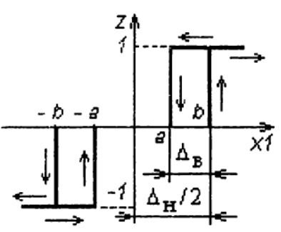
Nonlinear element model
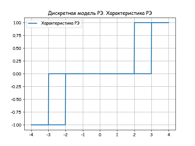
#!/usr/bin/env python #coding=utf8 import matplotlib.pyplot as plt import matplotlib as mpl mpl.rcParams['font.family'] = 'fantasy' mpl.rcParams['font.fantasy'] = 'Comic Sans MS, Arial' from numpy import arange,sin,cos,sign def z(t,a,b): if -a<4*sin(t)<b and 4*cos(t)>0: z=0 elif -b<4*sin(t)<a and 4*cos(t)<0: z=0 else: z=sign(sin(t)) return zx=arange(0,6,0.005) y=[4*sin(t) for t in x] y1=[z(t,2,3) for t in x] y2=[2 for t in x] y3=[3 for t in x] plt.figure() plt.title(' : -') plt.plot(x, y, linewidth=2, label=' ') plt.plot(x, y1, linewidth=2, label=' ') plt.plot(x, y2, linewidth=1, label='2 ') plt.plot(x, y3,linewidth=1, label='3') plt.legend(loc='best') plt.grid(True) plt.figure() plt.title(' . ') plt.plot(y, y1, linewidth=2, label=' ') plt.legend(loc='best') plt.grid(True) plt.show() Analyzing the result of the model on the following two graphs:
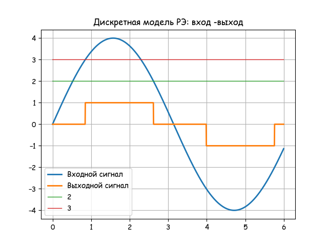
The discrete model of the OM is based on difference equations. Formative PI-algorithm feedback is implemented using aperiodic link with transfer function:
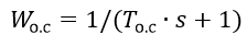
The control unit (RB) is a pulse width modulator (PWM) that can be built using both analog and digital means.
The control unit, together with the constant speed actuator, provides, under certain conditions, a fairly accurate implementation of the PI algorithm:
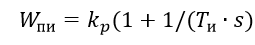 (one)
(one)And accordingly, the transient characteristics:
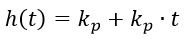 (2)
(2)To implement the PID algorithm , the differentiator W (s) is connected to the input of the PI controller of the relay-pulse action according to the scheme:
The introduced transfer W (s) is formed by one or two successively connected differentiating links. The control unit together with the constant speed actuator provides, under certain conditions, a fairly accurate implementation of the PID algorithm:
 (3)
(3)And accordingly, the transient characteristics:
 (four)
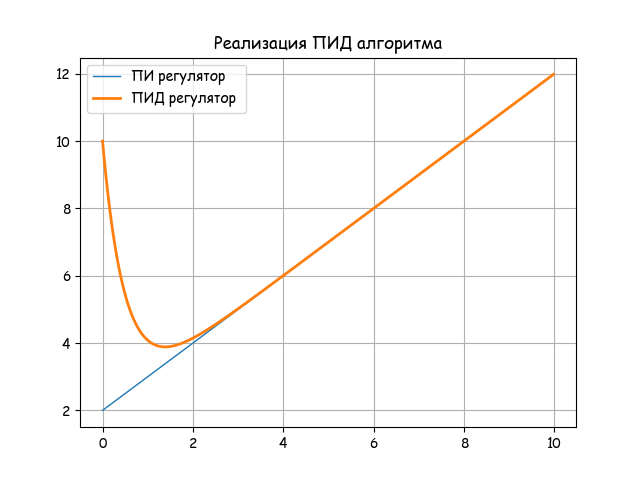
Listing for comparing PI and PID algorithms
#!/usr/bin/env python #coding=utf8 import matplotlib.pyplot as plt import matplotlib as mpl mpl.rcParams['font.family'] = 'fantasy' mpl.rcParams['font.fantasy'] = 'Comic Sans MS, Arial' from numpy import e,arange def hp(t,Kp,Ti,Kd,Td): z=Kp+Kp*t/Ti+Kp*Kd*e**(-t/Td) return z x=arange(0,10,0.02) y1=[hp(t,2,2,0,0.5) for t in x] y2=[hp(t,2,2,4,0.5) for t in x] plt.title(' ') plt.plot(x, y1, linewidth=1, label=' ') plt.plot(x, y2, linewidth=2, label=' ') plt.legend(loc='best') plt.grid(True) plt.show() Analyze the transient graph for the selected settings for PI and PID algorithms.
Linear models of relay-pulse regulators do not exclude the possibility of instantaneous changes in the regulating influence (output value of the regulator).
For real relay-pulse regulators, the displacement of the output shaft or the shaft of the EIM occurs in a certain finite time, depending on both the set values of the settings and the speed of the actuator so .
So, with a step change in the input signal, the pulse duration at the output of the RB control unit for the P-algorithm is determined by the relation:
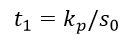
The duration of the first pulse at the output of the RB for the PI algorithm is determined by the equation:
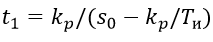
Subsequent pulses of constant duration t and are repeated at the following time intervals:
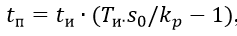
Where
 - the transmission coefficient of the regulator;
  - constant integration, with;
  - speed of the actuator,
  .
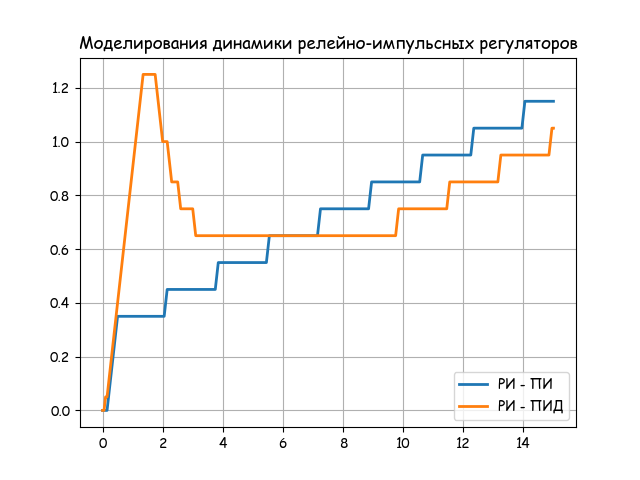
.3. Modeling of the dynamics of relay-pulse P-PI and PID-regulators in non-equilibrium modes
The graph of the relay-pulse PID controller is shown in the following figure:
Listing model of the dynamics of the relay-pulse regulators
#!/usr/bin/env python #coding=utf8 import matplotlib.pyplot as plt import matplotlib as mpl mpl.rcParams['font.family'] = 'fantasy' mpl.rcParams['font.fantasy'] = 'Comic Sans MS, Arial' from numpy import arange,sign def fd(Kd,Td,dt,x,x1,y):# - () return (1-dt/Td)*y+Kd*(x-x1) def fa(Ta,Ka,dt,x,y):# ( ) return (1-dt/Ta)*y+Ka*x*dt/Ta def fi(so,dt,x,y):# ( ) return y+so*x*dt """ """ te=15;N=300;dt=0.05 x0=[0 for w in arange(0,N+1)];x1=[0 for w in arange(0,N+1)] x2=[0 for w in arange(0,N+1)];x3=[0 for w in arange(0,N+1)] z=[0 for w in arange(0,N+1)];z1=[0 for w in arange(0,N+1)] z2=[0 for w in arange(0,N+1)];m=[0 for w in arange(0,N+1)] x=[0 for w in arange(0,N+1)] """ """ def P(so,Ka,Ta,a,b,Kd,Td,Dl,e): for j in arange(0,N,1): x0[j+1]=e-Dl*m[j] x[j+1]=x0[j+1]+x2[j]-x3[j] if -a<x[j+1]<b and x[j+1]>x[j]: z1[j+1]=0 else: z1[j+1]=sign(x[j-1]) if -b<x[j+1]<a and x[j+1]<x[j]: z2[j+1]=0 else: z2[j+1]=sign(x[j-1]) if x[j+1]>x[j]: z[j+1]=z1[j+1] else: z[j+1]=z2[j+1] x1[j+1]=fd(Kd,Td,dt,x0[j+1],x0[j],x1[j]) x2[j+1]=fd(1,Ta,dt,x1[j+1],x1[j],x2[j]) x3[j+1]=fa(Ta,Ka,dt,z[j+1],x3[j]) m[j+1]=fi(so,dt,z[j],m[j]) return m NN=[j*dt for j in arange(0,N+1,1)] #P(so,Ka,Ta,a,b,Kd,Td,Dl,e) #PID=P(1,10,5,0.4,0.5,10,1,0,1) #PP=P(1,0.1,0.1,0.2,0.6,0,0.2,4,1) #PI=P(1,10,5,0.4,0.5,0,0.2,0,1) #PI1=P(0.5,10,5,0.4,0.5,0,0.2,0,1) plt.figure() plt.title(' - ') plt.plot(NN, P(1,10,5,0.4,0.5,0,0.2,0,1), linewidth=2, label=' - ') plt.plot(NN,P(1,10,5,0.4,0.5,10,1,0,1), linewidth=2, label=' - ') plt.legend(loc='best') plt.grid(True) plt.figure() plt.title(' - ') plt.plot(NN, P(1,10,5,0.4,0.5,0,0.2,0,1), linewidth=2, label=' -. -1 -1') plt.plot(NN,P(0.5,10,5,0.4,0.5,0,0.2,0,1), linewidth=2, label=' -. -0.5 -1') plt.plot(NN,P(1,0.1,0.1,0.2,0.6,0,0.2,4,1), linewidth=2, label=' -. -1 -1') plt.legend(loc='best') plt.grid(True) plt.show() Analyzing the results.
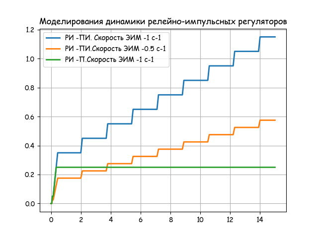
The characteristic of the regulator depends on the speed of the actuator so, and the parameters of the relay element a, b. The value of so is predetermined by the type of EIM and is characterized by the parameter Tim - the minimum time of a full stroke. For standard EIM, the Tim values are 10,25,63, 100 and 160 s.
The value of b (half dead band) is set by the maximum tolerance, to which the regulator should not react.
The settings of the controller Kp, Ti, Kd, Td are non-linearly dependent on the speed of the actuator so, the feedback parameters Ka, Ta and the relay element a, b.
findings
By means of the Python programming language, using the finite difference method, mathematical models of electronic relay-impulse controllers of indirect action are obtained.
The resulting models can be used in the design of microprocessor control devices.
Links
Source: https://habr.com/ru/post/345714/
All Articles