Data mining in R
This post is a translation of three parts of the Data acquisition in R series from my English-language blog . The original series is conceived in four parts, three of which formed the basis of this post: Use of prepared data sets ; Access to popular statistical databases ; Demographic data ; Demographic data . The final part that has not yet been written will deal with the use of spatial data.

R sharpened by reproducible results. There are many excellent solutions that ensure the compatibility of system versions and packages that help apply the principles of literate programming ... I want to show how you can easily and efficiently find / download / extract data using R itself and documenting each step, which ensures complete reproducibility of the entire process. Of course, I don’t set myself the task of listing all possible data sources and focusing mainly on demographic data. If your interests lie outside the scope of population statistics, it is worth looking in the direction of the magnificent Open Data Task View project.
To illustrate the use of each of the sources of information, I give an example of visualization of the data. Each code sample is designed as a separate unit — copy and reproduce. Of course, you first need to install the required packages. All code lies entirely here .
Embedded datasets
Many packages include small convenient data sets to illustrate the methods. Actually, the core of R includes the datasets package, which contains a large number of small, diverse, sometimes very famous, datasets. A detailed list of illustrative datasets embedded in various packages is provided on Vincent Arel-Bundock website .
A nice feature of embedded datasets is that they are "always with you." Unique training dataset names can be used as easily as any objects from the Global Environment. Let's take a look at the charming tiny dataset of swiss - Swiss Fertility and Socioeconomic Indicators (1888) Data. Below I will show the differences in the birth rate between the cantons of Switzerland depending on the proportion of the rural population and the prevalence of the Catholic faith.
library(tidyverse) swiss %>% ggplot(aes(x = Agriculture, y = Fertility, color = Catholic > 50))+ geom_point()+ stat_ellipse()+ theme_minimal(base_family = "mono") 
Gapminder
Some packages are specifically designed to make certain data sets easily accessible to users of R. A good example of such a package is gapminder , which contains an illustrative sample of Hapan Rosling's Gapminder project data.
library(tidyverse) library(gapminder) gapminder %>% ggplot(aes(x = year, y = lifeExp, color = continent))+ geom_jitter(size = 1, alpha = .2, width = .75)+ stat_summary(geom = "path", fun.y = mean, size = 1)+ theme_minimal(base_family = "mono") 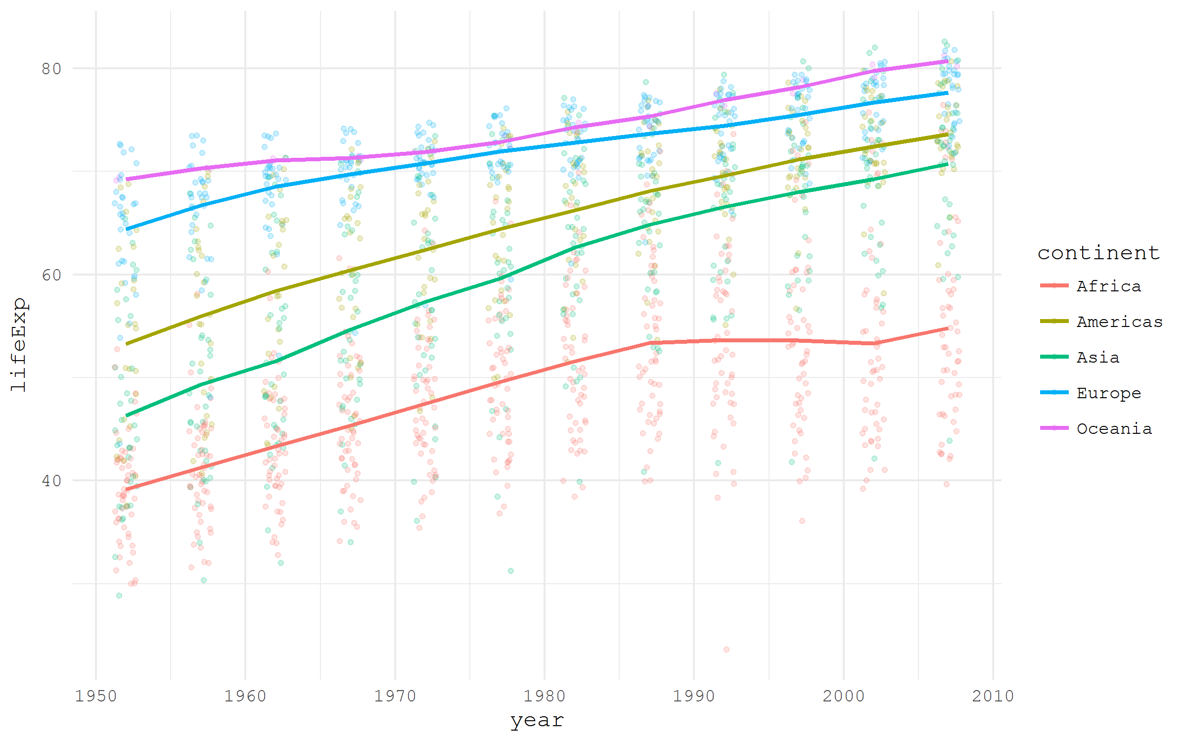
Dataset by URL
If a data set is stored somewhere online and has a direct link to download, it can be easily read in R, just by specifying a reference. For example, let's take the famous Galton dataset on the growth of fathers and children from the HistData package. Just take the data for a direct link from Vincent Arel-Bundock's list.
library(tidyverse) galton <- read_csv("https://raw.githubusercontent.com/vincentarelbundock/Rdatasets/master/csv/HistData/Galton.csv") galton %>% ggplot(aes(x = father, y = height))+ geom_point(alpha = .2)+ stat_smooth(method = "lm")+ theme_minimal(base_family = "mono") 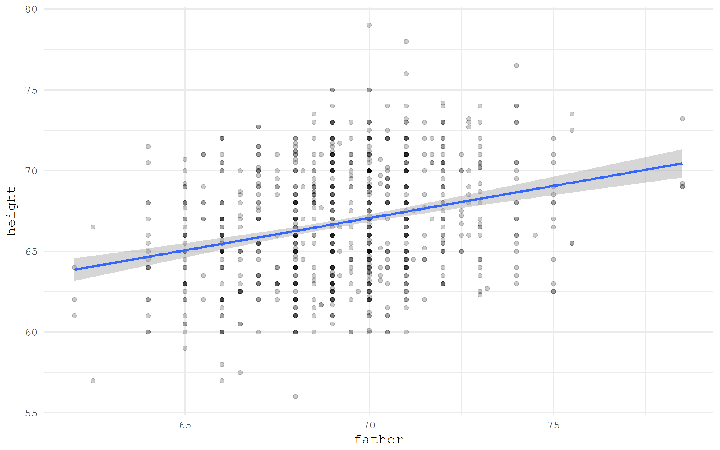
Download and unpack the archive
Very often, data sets are archived before being released to the Internet. Reading the archive immediately fails, but the solution in R is quite simple. The process logic is very simple: first we create a directory where we will unpack the data; then download the archive to a temporary file; Finally, unpack the archive into a previously created directory. For example, I download Historical New York City Crime Data , a set of data on crimes committed in New York, which was kindly provided by the State of New York and stored in the data data repository data.gov.
library(tidyverse) library(readxl) # create a directory for the unzipped data ifelse(!dir.exists("unzipped"), dir.create("unzipped"), "Directory already exists") # specify the URL of the archive url_zip <- "http://www.nyc.gov/html/nypd/downloads/zip/analysis_and_planning/citywide_historical_crime_data_archive.zip" # storing the archive in a temporary file f <- tempfile() download.file(url_zip, destfile = f) unzip(f, exdir = "unzipped/.") Sometimes the downloaded archive is weighty enough, and we would not want to download it again each time, playing the code. In this case, it makes sense to save the original archive, rather than use a temporary file.
# if we want to keep the .zip file path_unzip <- "unzipped/data_archive.zip" ifelse(!file.exists(path_unzip), download.file(url_zip, path_unzip, mode="wb"), 'file alredy exists') unzip(path_unzip, exdir = "unzipped/.") Finally, let's import and visualize the downloaded and unzipped data.
murder <- read_xls("unzipped/Web Data 2010-2011/Seven Major Felony Offenses 2000 - 2011.xls", sheet = 1, range = "A5:M13") %>% filter(OFFENSE %>% substr(1, 6) == "MURDER") %>% gather("year", "value", 2:13) %>% mutate(year = year %>% as.numeric()) murder %>% ggplot(aes(year, value))+ geom_point()+ stat_smooth(method = "lm")+ theme_minimal(base_family = "mono")+ labs(title = "Murders in New York") 
Figshare
In the academic world, the issue of reproducibility is becoming ever more acute. Therefore, more and more often openly published data sets become true companions of scientific articles. There are many specialized repositories for such data sets. One of the most widely used is Figshare. For him, there is a wrapper for R - rfigshare . For example, I download my own set of data about the growth of hockey players , which I collected for writing one of the previous posts on Habré . Please note that the first time you use the rfigshare package, you will be asked to enter the login and password from Figshare to access the API - a special web page will open in the browser.
There is a special function fs_search , but, in my experience, it is easier to find in the browser the data we are interested in and copy the unique identifier, by which we download it to R. The fs_download function turns the id into a direct link to download the file.
library(tidyverse) library(rfigshare) url <- fs_download(article_id = "3394735") hockey <- read_csv(url) hockey %>% ggplot(aes(x = year, y = height))+ geom_jitter(size = 2, color = "#35978f", alpha = .1, width = .25)+ stat_smooth(method = "lm", size = 1)+ ylab("height, cm")+ xlab("year of competition")+ scale_x_continuous(breaks = seq(2005, 2015, 5), labels = seq(2005, 2015, 5))+ theme_minimal(base_family = "mono") 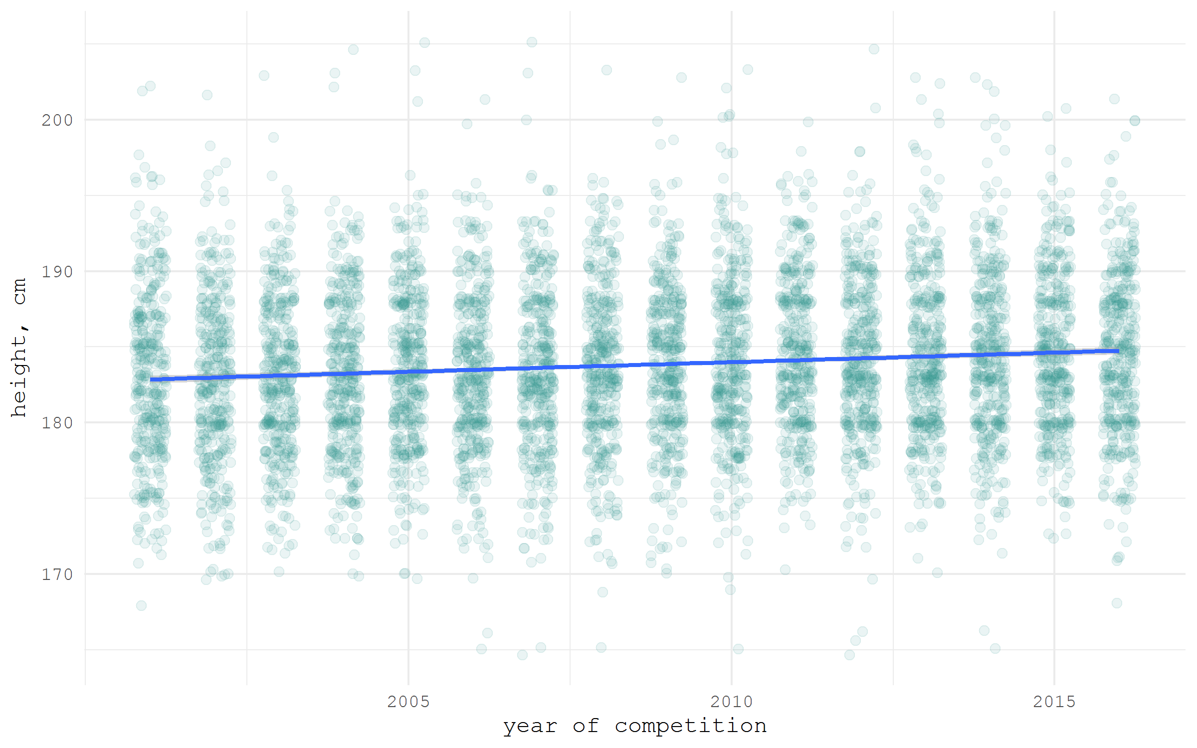
Eurostat
Eurostat publishes an unbelievable amount of statistics on European countries and their regions. Of course, there is a special package eurostat for all this wealth. Unfortunately, the built-in search_eurostat function search_eurostat not do well with the task of searching for relevant datasets. For example, on request life expectancy we get only two options, while in reality there should be several dozens of datasets. Therefore, the most convenient solution looks like this: go to the Eurostat website , find the data we are interested in, copy only its code and, finally, download it using the eurostat package. Please note that all Eurostat regional statistics are in a separate database .
I am now downloading data on life expectancy in European countries, the demo_mlexpec code is demo_mlexpec .
library(tidyverse) library(lubridate) library(eurostat) # download the selected dataset e0 <- get_eurostat("demo_mlexpec") Downloading may take some time, depending on the amount of dataset. In our case, we have a medium-sized set of 400K observations. If for some reason it is impossible to download datasets automatically (I have never had one), you can manually download it from a separate Eurostat website Bulk Download Service .
Let's look at the residual life expectancy at the age of 65 years in some selected European countries, separately for men and women. The age of 65 is the most common traditional retirement age. Look at the residual life expectancy for this age in the dynamics is very interesting in light of the talk about the reforms of the retirement age. From the downloaded data, we select only estimates of residual life expectancy at the age of 65, then we filter only estimates separately for men and women, finally, we leave only a few countries: Germany, France, Italy, Russia, Spain and the UK.
e0 %>% filter(! sex == "T", age == "Y65", geo %in% c("DE", "FR", "IT", "RU", "ES", "UK")) %>% ggplot(aes(x = time %>% year(), y = values, color = sex))+ geom_path()+ facet_wrap(~ geo, ncol = 3)+ labs(y = "Life expectancy at age 65", x = NULL)+ theme_minimal(base_family = "mono") 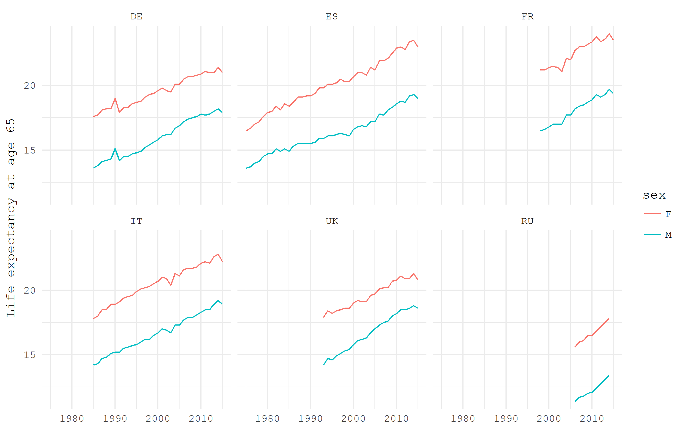
World Bank
There are several packages that provide access to World Bank data from R. Probably the most finished one is pretty fresh wbstats . Its wbsearch function really does an excellent job with finding the relevant datasets. For example, wbsearch("fertility") gives an explanatory list of 339 indicators in the form of a convenient table.
library(tidyverse) library(wbstats) # search for a dataset of interest wbsearch("fertility") %>% head | indicatorID | indicator | |
|---|---|---|
| 2479 | SP.DYN.WFRT.Q5 | Total wanted fertility rate (births per woman): Q5 (highest) |
| 2480 | SP.DYN.WFRT.Q4 | Total wanted fertility rate (births per woman): Q4 |
| 2481 | SP.DYN.WFRT.Q3 | Total wanted fertility rate (births per woman): Q3 |
| 2482 | SP.DYN.WFRT.Q2 | Total wanted fertility rate (births per woman): Q2 |
| 2483 | SP.DYN.WFRT.Q1 | Total wanted fertility rate (births per woman): Q1 (lowest) |
| 2484 | SP.DYN.WFRT | Wanted fertility rate (births per woman) |
Let's look at the indicator Lifetime risk of maternal death (%) (code SH.MMR.RISK.ZS ) - the risk of death for a woman throughout her life associated with the birth of children. The World Bank provides data by country, as well as several different groupings of countries. One of the notable options for grouping is the separation according to the principle of completeness of the Demographic Transition. Below I show the selected indicator for (1) countries that have already completed the CAP, (2) countries that have not yet completed the CAP, and (3) the world as a whole.
# fetch the selected dataset df_wb <- wb(indicator = "SH.MMR.RISK.ZS", startdate = 2000, enddate = 2015) # have look at the data for one year df_wb %>% filter(date == 2015) %>% View df_wb %>% filter(iso2c %in% c("V4", "V1", "1W")) %>% ggplot(aes(x = date %>% as.numeric(), y = value, color = country))+ geom_path(size = 1)+ scale_color_brewer(NULL, palette = "Dark2")+ labs(x = NULL, y = NULL, title = "Lifetime risk of maternal death (%)")+ theme_minimal(base_family = "mono")+ theme(panel.grid.minor = element_blank(), legend.position = c(.8, .9)) 
OECD
The Organization for Economic Cooperation and Development (OECD) publishes a lot of data on the economic and demographic development of member countries. The OECD package greatly simplifies the use of this data in R. The search_dataset function search_dataset good job of finding the necessary data by keywords, and get_dataset loads the selected data. In the following example, I download data on the duration of unemployment periods and display this data for the male population of EU16, EU28 and the United States using the heatmap visualization method.
library(tidyverse) library(viridis) library(OECD) # search by keyword search_dataset("unemployment") %>% View # download the selected dataset df_oecd <- get_dataset("AVD_DUR") # turn variable names to lowercase names(df_oecd) <- names(df_oecd) %>% tolower() df_oecd %>% filter(country %in% c("EU16", "EU28", "USA"), sex == "MEN", ! age == "1524") %>% ggplot(aes(obstime, age, fill = obsvalue))+ geom_tile()+ scale_fill_viridis("Months", option = "B")+ scale_x_discrete(breaks = seq(1970, 2015, 5) %>% paste)+ facet_wrap(~ country, ncol = 1)+ labs(x = NULL, y = "Age groups", title = "Average duration of unemployment in months, males")+ theme_minimal(base_family = "mono") 
Wid
The World Wealth and Income Database is a harmonized series of data on inequality in income and wealth. The database developers took care of creating a special R package, which is currently available only on github .
library(tidyverse) #install.packages("devtools") devtools::install_github("WIDworld/wid-r-tool") library(wid) The function for downloading data is download_wid() . In order to correctly specify the arguments for downloading data, you will have to dig into the package documentation a bit and understand the rather complex variable coding system.
?wid_series_type ?wid_concepts The given example is adapted from a package vignette . It displays the share of wealth owned by the richest 1% and 10% of the population in France and the UK.
df_wid <- download_wid( indicators = "shweal", # Shares of personal wealth areas = c("FR", "GB"), # In France an Italy perc = c("p90p100", "p99p100") # Top 1% and top 10% ) df_wid %>% ggplot(aes(x = year, y = value, color = country)) + geom_path()+ labs(title = "Top 1% and top 10% personal wealth shares in France and Great Britain", y = "top share")+ facet_wrap(~ percentile)+ theme_minimal(base_family = "mono") 
Human mortality database
When it comes to checking the big questions about the laws of the dynamics of human populations, there is no more reliable source of information than the Human Mortality Database . This database is developed and maintained by demographers who apply state-of-the-art methodology to harmonize source data. The HMD Method Protocol is a masterpiece of demographic data methodology. The downside is that baseline data of sufficiently high quality are available only for a relatively small number of countries. To familiarize myself with user-accessible data, I heartily recommend the [Human Mortality Database Explorer] [exp], created by Jonas Schöley .
Thanks to Tim Riffe , we have the HMDHFDplus package, which allows you to load HMD data directly into R with just a few lines of code. Please note that you will need a free mortality.org account to access the data. As the name suggests, the package also allows you to download data from the equally beautiful Human Fertility Database .
The example below is taken from my previous post and has been updated a little. It seems to me that it illustrates well the power of automatic data download to R. Easily and naturally I download one-year age structures for all HMD countries for all available years, separately for women and men. When playing this code, it is worth remembering that several tens of megabytes of data will be downloaded. Next, I will calculate and map the sex ratio at all ages for all countries in 2012. Sex ratios reflect two key demographic patterns: 1) more boys are always born; 2) male mortality is higher than female mortality at all ages. Except for a few well-studied examples, the sex ratio at birth is 105-106 boys per 100 girls. Thus, significant differences in age profiles of the sex ratio reflect primarily gender differences in mortality.
# load required packages library(HMDHFDplus) library(tidyverse) library(purrr) # help function to list the available countries country <- getHMDcountries() # remove optional populations opt_pop <- c("FRACNP", "DEUTE", "DEUTW", "GBRCENW", "GBR_NP") country <- country[!country %in% opt_pop] # temporary function to download HMD data for a simgle county (dot = input) tempf_get_hmd <- . %>% readHMDweb("Exposures_1x1", ik_user_hmd, ik_pass_hmd) # download the data iteratively for all countries using purrr::map() exposures <- country %>% map(tempf_get_hmd) # data transformation to apply to each county dataframe tempf_trans_data <- . %>% select(Year, Age, Female, Male) %>% filter(Year %in% 2012) %>% select(-Year) %>% transmute(age = Age, ratio = Male / Female * 100) # perform transformation df_hmd <- exposures %>% map(tempf_trans_data) %>% bind_rows(.id = "country") # summarize all ages older than 90 (too jerky) df_hmd_90 <- df_hmd %>% filter(age %in% 90:110) %>% group_by(country) %>% summarise(ratio = ratio %>% mean(na.rm = T)) %>% ungroup() %>% transmute(country, age = 90, ratio) # insert summarized 90+ df_hmd_fin <- bind_rows(df_hmd %>% filter(!age %in% 90:110), df_hmd_90) # finaly - plot df_hmd_fin %>% ggplot(aes(age, ratio, color = country, group = country))+ geom_hline(yintercept = 100, color = "grey50", size = 1)+ geom_line(size = 1)+ scale_y_continuous(limits = c(0, 120), expand = c(0, 0), breaks = seq(0, 120, 20))+ scale_x_continuous(limits = c(0, 90), expand = c(0, 0), breaks = seq(0, 80, 20))+ facet_wrap(~country, ncol = 6)+ theme_minimal(base_family = "mono", base_size = 15)+ theme(legend.position = "none", panel.border = element_rect(size = .5, fill = NA, color = "grey50"))+ labs(x = "Age", y = "Sex ratio, males per 100 females", title = "Sex ratio in all countries from Human Mortality Database", subtitle = "HMD 2012, via HMDHFDplus by @timriffe1", caption = "ikashnitsky.imtqy.com") 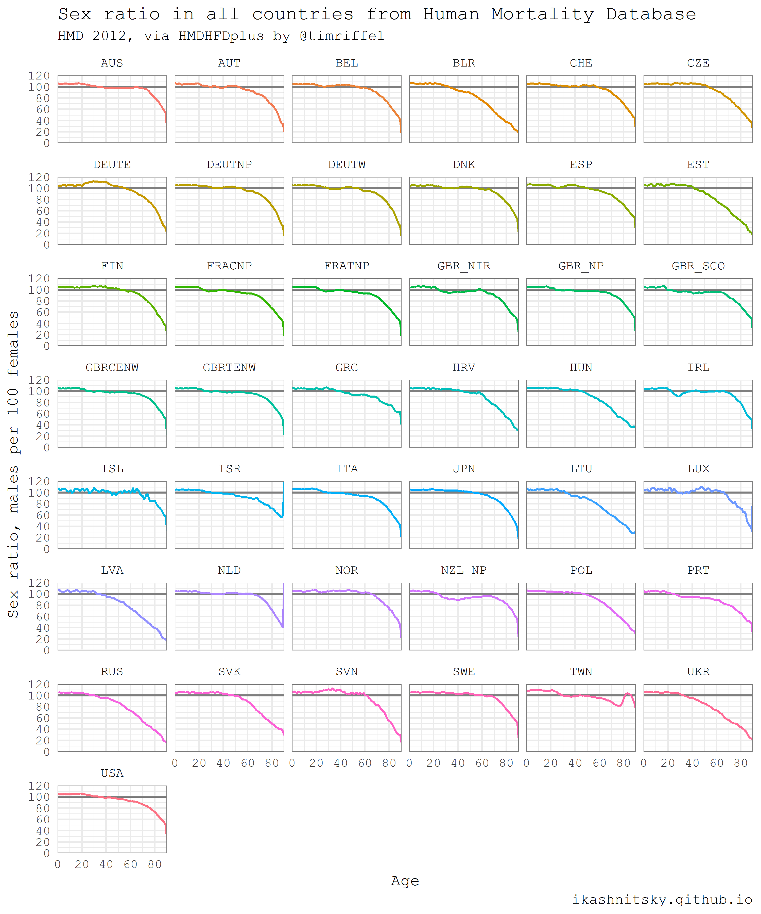
United Nations World Population Prospects
The UN Population Department publishes high-quality estimates and population projections for all countries of the world. Calculations are updated every 2-3 years and are published in the public domain as an interactive report World Population Prospects . These reports contain very general descriptive analysis and, of course, rich data. The data is available in R in special packages that have names like wpp20xx . To date, data is available for releases of 2008, 2010, 2012, 2015, and 2017. Here I will give an example of using wpp2015 data, taken from my previous post .
Using the ridgeplot visualization type, which received viral popularity this summer (under the previous, now rejected , ggjoy ) this summer thanks to the brilliant ggridges Claus Wilke package, I will show an impressive convergence of life expectancy at birth for men in the world since 1950.
library(wpp2015) library(tidyverse) library(ggridges) library(viridis) # get the UN country names data(UNlocations) countries <- UNlocations %>% pull(name) %>% paste # data on male life expectancy at birth data(e0M) e0M %>% filter(country %in% countries) %>% select(-last.observed) %>% gather(period, value, 3:15) %>% ggplot(aes(x = value, y = period %>% fct_rev()))+ geom_density_ridges(aes(fill = period))+ scale_fill_viridis(discrete = T, option = "B", direction = -1, begin = .1, end = .9)+ labs(x = "Male life expectancy at birth", y = "Period", title = "Global convergence in male life expectancy at birth since 1950", subtitle = "UNPD World Population Prospects 2015 Revision, via wpp2015", caption = "ikashnitsky.imtqy.com")+ theme_minimal(base_family = "mono")+ theme(legend.position = "none") 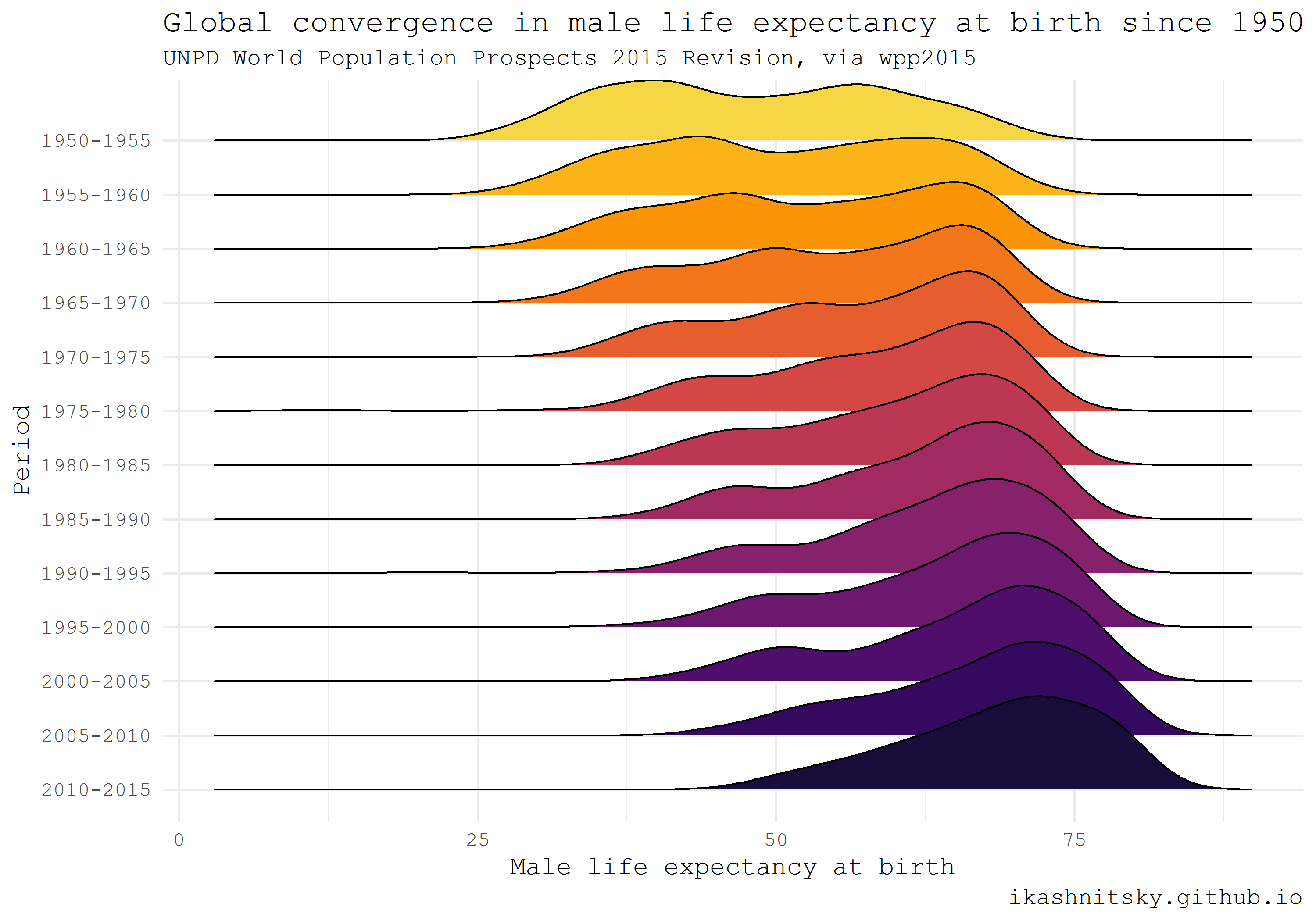
European Social Survey (ESS)
The European Social Survey publishes uniquely detailed data on European values, representative at country level and comparable across countries. Every two years, another wave of surveys is conducted in each of the participating countries. Data is available after free registration . Datasets are distributed in finished form for analysis using SAS, SPSS, or STATA. Thanks to Jorge Cimentada, we now have the opportunity to get this data in ready form and in R using the ess package. I will show how respondents assessed their level of trust in local police in all countries that participated in the latest survey wave.
library(ess) library(tidyverse) # help gunction to see the available countries show_countries() # check the available rounds for a selected country show_country_rounds("Netherlands") # get the full dataset of the last (8) round df_ess <- ess_rounds(8, your_email = ik_email) # select a variable and calculate mean value df_ess_select <- df_ess %>% bind_rows() %>% select(idno, cntry, trstplc) %>% group_by(cntry) %>% mutate(avg = trstplc %>% mean(na.rm = T)) %>% ungroup() %>% mutate(cntry = cntry %>% as_factor() %>% fct_reorder(avg)) df_ess_select %>% ggplot(aes(trstplc, fill = avg))+ geom_histogram()+ scale_x_continuous(limits = c(0, 11), breaks = seq(2, 10, 2))+ scale_fill_gradient("Average\ntrust\nscore", low = "black", high = "aquamarine")+ facet_wrap(~cntry, ncol = 6)+ theme_minimal(base_family = "mono")+ labs(x = "Trust score [0 -- 10]", y = "# of respondents", title = "Trust in police", subtitle = "ESS wave 8 2017, via ess by @cimentadaj", caption = "ikashnitsky.imtqy.com") 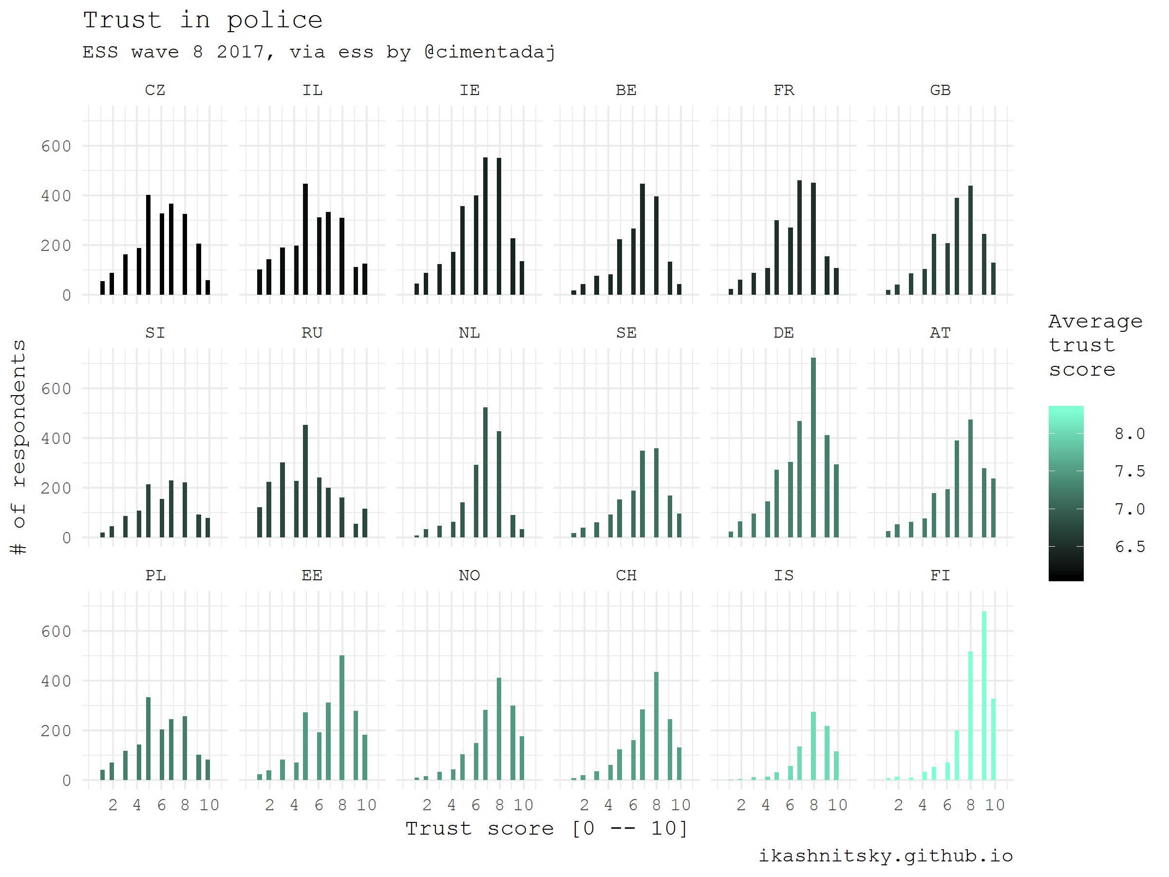
American Community Survey and Census
Immediately, several packages provide access to US census data and regular household sample surveys (American Community Survey). Probably the most beautiful implementation created recently by Kyle Walker - tidycensus . The Kill-feature of this package is the ability to download spatial data along with statistical data. Spatial data is downloaded as simple features, a revolutionary approach to geodata in R, recently introduced in the sf Edzer Pebesma package . This approach will accelerate the processing of a few dozen times, while simplifying the code to impossibility. But the details - in the final post of the series. Please note that in order to render simple features we need to install the development version of the ggplot2 package.
The map below shows the median age of the population in the census trails of the city of Chicago according to ACS data for 2015. To extract this data using tidycensus will first need to get an API key, which can be easily done when registering here .
library(tidycensus) library(tidyverse) library(viridis) library(janitor) library(sf) # to use geom_sf we need the latest development version of ggplot2 devtools::install_github("tidyverse/ggplot2", "develop") library(ggplot2) # you need a personal API key, available free at # https://api.census.gov/data/key_signup.html # normally, this key is to be stored in .Renviron # see state and county codes and names fips_codes %>% View # the available variables load_variables(year = 2015, dataset = "acs5") %>% View # data on median age of population in Chicago df_acs <- get_acs( geography = "tract", county = "Cook County", state = "IL", variables = "B01002_001E", year = 2015, key = ik_api_acs, geometry = TRUE ) %>% clean_names() # map the data df_acs %>% ggplot()+ geom_sf(aes(fill = estimate %>% cut(breaks = seq(20, 60, 10))), color = NA)+ scale_fill_viridis_d("Median age", begin = .4)+ coord_sf(datum = NA)+ theme_void(base_family = "mono")+ theme(legend.position = c(.15, .15))+ labs(title = "Median age of population in Chicago\nby census tracts\n", subtitle = "ACS 2015, via tidycensus by @kyle_e_walker", caption = "ikashnitsky.imtqy.com", x = NULL, y = NULL) 
Enjoy your journey to the world of open data with R!
')
Source: https://habr.com/ru/post/345664/
All Articles