Volumetric atmospheric light scattering
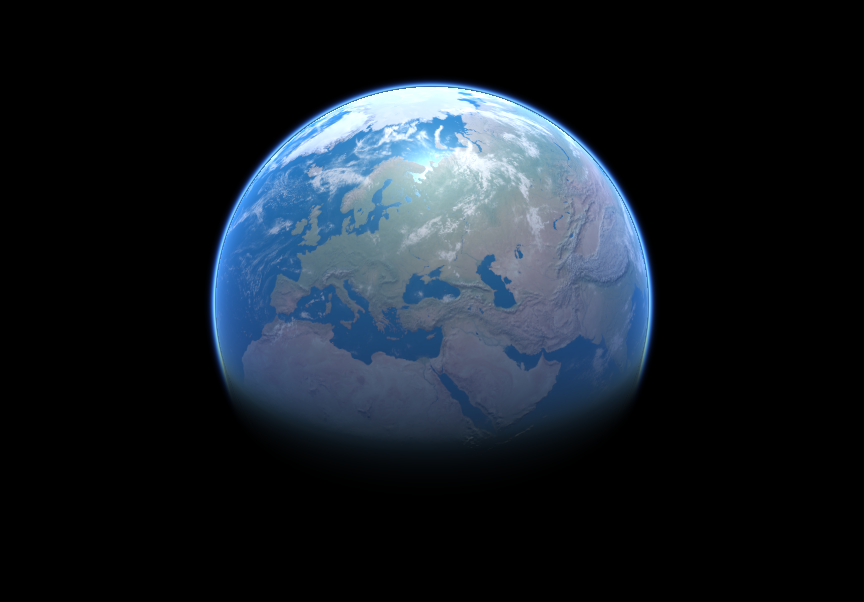
If you have lived on planet Earth long enough, then you probably wondered why the sky is usually blue, but it turns red at sunset. The optical phenomenon that has become the (main) cause of this is called Rayleigh scattering . In this article I will explain how to model atmospheric scattering to simulate many of the visual effects that appear on planets. If you want to learn how to render physically accurate images of alien planets, then this tutorial is definitely worth studying.
The article is divided into the following parts:
- Part 1. Volumetric atmospheric scattering.
- Part 2. The Theory of Atmospheric Scattering
- Part 3. Mathematics of Rayleigh Scattering
- Part 4. Journey through the atmosphere
- Part 5. Atmospheric shader
- Part 6. Crossing the atmosphere
- Part 7. Atmospheric Scatter Shader
Part 1. Volumetric atmospheric scattering.
Introduction
Recreating atmospheric phenomena is so difficult because the sky is not an opaque object. In traditional rendering techniques, it is assumed that the objects are just empty shells. All graphic calculations are performed on the surfaces of materials and do not depend on what is inside. This strong simplification allows for very efficient rendering of opaque objects. However, the properties of some materials are determined by the fact that light can pass through them. The final appearance of translucent objects becomes the result of the interaction of light with their internal structure. In most cases, this interaction can be very effectively imitated, as can be seen in the tutorial " Fast Shader for Subsurface Scattering in Unity ". Unfortunately, in our case, if we want to create a convincing sky, this is not so. Instead of rendering only the “outer shell” of the planet, we will have to simulate what happens to the rays of light passing through the atmosphere. Performing calculations inside an object is called volume rendering ; We discussed this topic in detail in a series of articles, Volumetric Rendering . In this series of articles, I talked about two techniques ( raymarching and iconic distance functions ) that cannot be effectively used to simulate atmospheric scattering. In this article, we will introduce a technique that is more suitable for rendering translucent solid objects, often called unit volume scattering .
')
Single scatter
In a room without light, we will not see anything. Objects become visible only when the rays of light are reflected from them and enter our eye. Most game engines (such as Unity and Unreal) assume that the light moves in a “vacuum”. This means that only objects can affect the light. In fact, the light always moves in the environment. In our case, this medium is the air we breathe. Therefore, the distance traveled by light in the air affects the appearance of the object. On the surface of the Earth, the density of air is relatively small, its influence is so insignificant that it should be considered only when light travels long distances. Distant mountains merge with the sky, but atmospheric scattering has almost no effect on nearby objects.
The first step in recreating the optical effect of atmospheric scattering is to analyze how light passes through environments such as air. As stated above, we can see an object only when light falls into our eyes. In the context of 3D graphics, our eye is the camera used to render the scene. The molecules that make up the air around us can reflect the light rays passing through them. Therefore, they are able to change the way we perceive objects. If to simplify greatly, then there are two ways in which molecules can affect our vision.
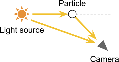
Scattering out
The most obvious way of interacting molecules with light is that they reflect light, changing its direction. If the light beam directed into the camera is reflected, then we observe the scattering process outside .

A real source of light can emit quadrillion photons every second, and each of them with a certain probability can collide with an air molecule. The denser the environment in which the light moves, the more likely the reflection of a single photon. The effect of scattering outside also depends on the distance traveled by the light.
Scattering outward causes the light to gradually become dimmer, and this property depends on the distance traveled and the density of the air.
Inward scattering
When a light is reflected by a particle, it may happen that it is redirected to the camera. Such an effect is the opposite of scattering out, and it is logical that it is called scattering inward .
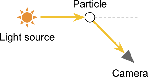
Under certain conditions, scattering inside allows you to see light sources that are not in the direct field of view of the camera. The most obvious result of this is an optical effect - light halos around light sources. They arise from the fact that the camera receives from one source both direct and indirect rays of light, which de facto increases the number of photons produced.
Unit volume scattering
One ray of light can be reflected any number of times. This means that before you get into the camera. the beam can pass very difficult routes. This becomes a serious difficulty for us, because the rendering of high-quality translucent materials requires the simulation of the paths of each of the individual rays of light. This technique is called raytracing , and is currently too expensive to implement in real time. The single scattering technique presented in this tutorial takes into account a single event of scattering a ray of light. Later we will see that such a simplification still allows to obtain realistic results in just a small fraction of the calculations required for true ray tracing.
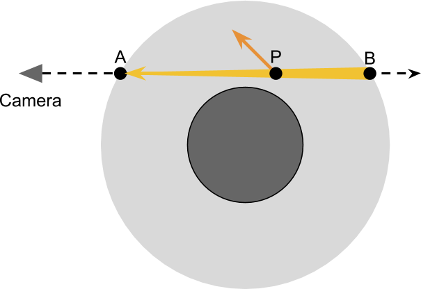
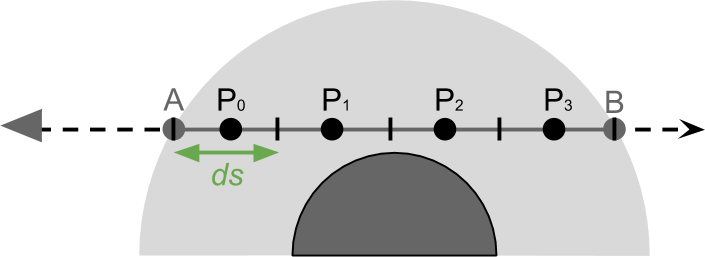
The basis for rendering a realistic sky is a simulation of what happens to the rays of light as it passes through the atmosphere of the planet. The diagram below shows a camera looking through the planet. The main idea of this rendering technique is to calculate how the passage of light from A at B affects scattering. This means that it is necessary to calculate the influence that scattering in and out on the beam passing to the camera has. As stated above, due to scattering outward, we observe attenuation. The amount of light present at each point P i n o v e r l i n e a b has a small chance of reflection away from the camera.
To correctly take into account the amount of scattering outward, occurring at each point P we first need to know how much light was present in P . If we assume that only one star illuminates the planet, then all the light received P should come from the sun. Part of this light will be scattered inward and reflected into the camera:
These two stages are sufficient to approximate most of the effects observed in the atmosphere. However, everything is complicated by the fact that the amount of light produced P from the sun is also subject to scattering when the light passes through the atmosphere from C at P .

To summarize what we need to do:
- The field of view of the camera enters the atmosphere in A and is in B ;
- As an approximation, we will take into account the influence of inward and outward scattering when it occurs at each point P i n o v e r l i n e a b ;
- The amount of light received P from the sun;
- The amount of light received P and scattered to the outside as it passes through the atmosphere o v e r l i n e C P ;
- Part of the light received P and scattered inward, which redirects the rays to the camera;
- Part of the world of P sent to the camera, scattered outward and reflected from the field of view.
However, there are many ways in which rays can enter the camera. For example, one of the rays, scattered outwards on the way to P , in a second collision, it can be scattered back towards the camera (see diagram below). And there may be rays reaching the camera after three reflections, or even four.

The technique we are considering is called unit scattering , because it takes into account only inward scattering that occurs along the field of view. More sophisticated techniques can expand this process and take into account other ways the beam can reach the camera. However, the number of possible paths increases exponentially with the number of scattering events considered. Fortunately, the probability of hitting the camera also decreases exponentially.
Part 2. The Theory of Atmospheric Scattering
In this part, we will begin to derive the equations that control this complex, but wonderful optical phenomenon.
Pass function
To calculate the amount of light transmitted to the camera, it is useful to make the same journey that the rays from the sun pass. Looking at the diagram below, it is easy to see that the rays of light reaching C pass through the empty space. Since there is nothing on their way, all the light reaches C without undergoing any scattering effect. Let's mark the variable I C the amount of unscattered light produced by a point C from the sun. During his journey to P , the ray enters the atmosphere of the planet. Some rays collide with molecules hanging in the air and are reflected in different directions. As a result, part of the light is scattered from the path. Amount of light reaching P (denoted as I P ) will be less than I C .

Ratio I C and I P called transmittance :
T l e f t ( o v e r l i n e C P r i g h t ) = f r a c I P I C
We can use it to denote the percentage of light that was not scattered (that is, was missed ) when traveling from C before P . Later we explore the nature of this function. So far the only thing we need to know is that it corresponds to the influence of atmospheric dispersion to the outside.
Therefore, the amount of light produced P equals:
I P = I CT l e ft( overlineCP right)
Scatter function
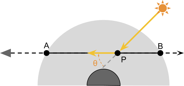
Point P receives light directly from the sun. However, not all of this light passing through P transferred back to the camera. To calculate the amount of light actually reaching the camera, we introduce a new concept: the scattering function S . It will denote the amount of light reflected in a particular direction. If we look at the diagram below, we will see that only the rays reflected at the angle will be directed to the camera. theta .
Value S l e f t ( l ambda, theta,h right) denotes the fraction of light reflected on theta radian. This function is our main problem, and we explore its nature in the next section. So far the only thing you need to know is that it depends on the color of the light produced (determined by the wavelength lambda ), scattering angle theta and heights h points P . Altitude is important because the density of the atmosphere varies as a function of altitude. And density is one of the factors determining the amount of light scattered.
We now have all the necessary tools to write a general equation showing the amount of light transmitted from P to A :
IPA= boxedIPS l e f t ( l a mbda, theta,h right)T l e f t ( o v e rlinePA right)
Thanks to the previous definition, we can deploy IP :
IPA= boxedICT l e f t ( overlineCP right)S l e f t ( l a m b da, theta,h right)T l e f t ( o v e r linePA right)=
= underset textin−scattering underbraceICS left( lambda, theta,h right) underset textout−scattering underbraceT left( overlineCP right)T left( overlinePA right)
The equation speaks for itself:
- Light travels from the sun to C without dissipating in the vacuum of space;
- Light enters the atmosphere and passes from C to P . In this process, due to scattering outwardly only a part T left( overlineCP right) reaches destination;
- The part of the world that got from the sun to P Reflected back into the camera. The proportion of light subject to scattering is equal to S left( lambda, theta,h right) ;
- The remaining light passes from P before A and again only part T left( overlinePA right) .
Numerical integration
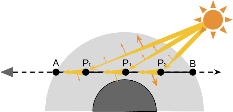
If you carefully read the previous paragraphs, you might have noticed that the brightness was recorded differently. Symbol IPA denotes the amount of light transmitted from P to A . However, the value does not take into account all the light that gets A . In these simplified models of atmospheric scattering, we take into account scattering inward from each point along the camera's field of view in the atmosphere.
Total amount of light received A ( IA ), calculated by adding the influence of all points P in overlineab . From the point of view of mathematics, on the segment overlineAB there is an infinite number of points, therefore a cyclic round of them is impossible. However, we can share overlineAB into smaller lengths ds (see diagram below), and summarize the influence of each of them.
Such an approximation process is called numerical integration and leads to the following expression:
IA= sumP in overlineABIPAds
The more points we take into account, the more accurate the final result will be. In reality, in our atmospheric shader, we simply loop around a few points. Pi inside the atmosphere, summing up their influence in the overall result.
You can look at it in another way: multiplying by d s , we "average" the influence of all points.
Directional lighting
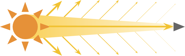
If the sun is relatively close, then it is best modeled as a point source of light . In this case, the amount received C light depends on the distance to the sun. However, if we are talking about planets, we often assume that the sun is so far away that its rays fall on the planet from one angle. If this is true, then we can simulate the sun as a directional light source . The light received from a directional light source remains constant, regardless of the distance traveled by it. Therefore every point C receives the same amount of light, and the direction relative to the sun is the same for all points.
We can use this assumption to simplify our equations.
Let's replace IC constant IS which determines the brightness of the sun .
IA= sumP in overlineAB boxedIPAds=
= sumP in overlineAB boxedICS left( lambda, theta,h right)T left( overlineCP right) ,T left( overlinePA right)ds=
=IS sumP in overlineABS left( lambda, theta,h right)T left( overlineCP right)T left( overlinePA right)ds=
There is one more optimization that we can perform, it includes the scattering function S left( lambda, theta,h right) . If sunlight always falls from one direction, then the angle theta becomes permanent. Below we will see that directional influence can be excluded from the amount. S left( lambda, theta,h right) . But for the time being we will leave him.
Absorption coefficient
In describing the possible results of the interaction between light and air molecules, we allowed only two options - either passing through or reflecting. But there is a third possibility. Some chemical compounds absorb light. In the atmosphere of the Earth there are many substances with this property. Ozone, for example, is located in the upper atmosphere and actively interacts with ultraviolet radiation. However, its presence has virtually no effect on the color of the sky, because it absorbs light outside the visible spectrum. Here on Earth, the influence of light-absorbing substances is often ignored. But in the case of other planets it is impossible to refuse him. For example, the usual coloring of Neptune and Uranus is caused by the presence of a large amount of methane in their atmosphere. Methane absorbs red light, which gives a blue hue. In the remaining part of the tutorial, we will ignore the absorption coefficient, but we will add a way to tint the atmosphere.
If you look at the colors of the visible spectrum (below), then it is easy to see that if enough blue light is scattered, then the sky can actually turn yellow or red.

There is a temptation to say that the color of the sky is associated with a shade of yellow Sahara sand. However, the same effect can be seen during large fires due to smoke particles, which are usually close to black.
Part 3. Mathematics of Rayleigh scattering.
In this part we will get acquainted with the mathematics of Rayleigh scattering - an optical phenomenon, because of which the sky looks blue. The equations derived in this part are transferred to the shader code of the next part.
Introduction
In the previous section, we derived an equation, which is a good basis for approximating atmospheric scatter in a shader. However, we missed the fact that a single equation does not give us convincing results. If we need a beautiful looking, atmospheric shader, then we need to delve a bit into math.
The interaction between light and matter is incredibly difficult, and we will not be able to fully describe it in an easy way. In fact, modeling atmospheric dispersion is very time consuming. Part of the problem is caused by the fact that the atmosphere is not a homogeneous medium. Its density and composition vary considerably as a function of height, which makes it almost impossible to create an “ideal” model.
That is why in the scientific literature there are several models of scattering, each of which is intended to describe a subset of optical phenomena that occur under certain conditions. Most of the optical effects demonstrated by the planets can be recreated, considering only two different models: Rayleigh scattering and light scattering by a spherical particle . These two mathematical tools allow us to predict the scattering of light on objects of different sizes. The first models the reflection of light by molecules of oxygen and nitrogen, which constitute most of the composition of the air. The latter models the reflection of light in larger structures present in the lower layers of the atmosphere, such as pollen, dust and pollutants.
Rayleigh scattering causes blue skies and red sunsets. The scattering of light by a spherical particle gives the clouds their white color. If you want to know how this happens, then we will have to dive deeper into the mathematics of scattering.
Rayleigh scattering
What is the fate of a photon hitting a particle? To answer this question, we need to rephrase it more formally. Imagine that a ray of light passes through empty space and suddenly collides with a particle. The result of such a collision strongly depends on the particle size and the color of the light beam. If the particle is small enough (about the size of atoms or molecules), then the behavior of light is better predicted using Rayleigh scattering .
What is going on? Part of the world continues on its way, “not feeling” any influence. However, a small percentage of this source light interacts with the particle and scatters in all directions. However, not all directions receive the same amount of light. The photons are more likely to pass right through the particle or are reflected back. That is, the photon reflection variant is 90 degrees less. This behavior can be seen in the diagram below. The blue line shows the most probable directions of stray light.

This optical phenomenon is mathematically described by the Rayleigh scattering equation. S left( lambda, theta,h right) which gives us a share of the original light I0 reflected in direction theta :
I=I0S left( lambda, theta,h right)
S left( lambda, theta,h right)= frac pi2 left(n2−1 right)22 underset textdensity underbrace frac rho left(h right)N overset textwavelength overbrace frac1 lambda4 underset textgeometry underbrace left(1+ cos2 theta right)
Where:
- lambda : wavelength (wavelength) of the incoming light;
- theta : scattering angle ;
- h : altitude of a point;
- n=1.00029 : air refractive index ;
- N=2.504 cdot1025 : number of molecules per cubic meter of standard atmosphere;
- rho left(h right) : density coefficient . This number at sea level is 1 , and exponentially decreases with increasing h . Much can be said about this function, and we will look at it in the following sections.
The equation used in this tutorial is taken from the Scientific article “ Taking into Account Atmospheric Scattering , Nishita et al.
If you are still interested in understanding why particles of light are so strangely reflected from air molecules, then the following explanation can provide an intuitive understanding of what is happening.
The cause of Rayleigh scattering is in fact not the “repulsion” of particles. Light is an electromagnetic wave, and it can interact with a charge imbalance present in certain molecules. These charges are saturated by absorbing the resulting electromagnetic radiation, which is later emitted again. The angular shape shown in the angular function shows how air molecules become electrical dipoles radiating like microscopic antennas.
The first thing that can be noticed in Rayleigh scattering is that more light travels in some directions than in others. The second important aspect is that the amount of scattered light strongly depends on the wavelength lambda the coming light. The pie chart shown below visualizes S left( lambda, theta,0 right) for three different wavelengths. Calculation S at h=0 often called sea level scattering .

The figure below shows the visualization of the scattering coefficients for a continuous range of wavelengths / colors of the visible spectrum (code is available in ShaderToy ).
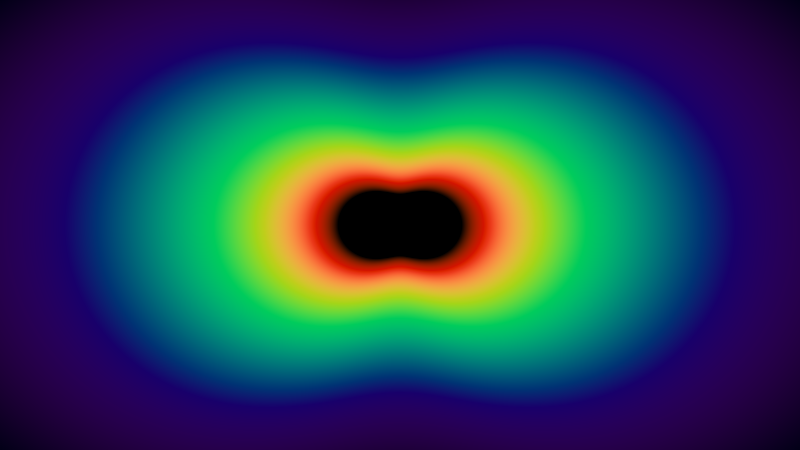
The center of the image looks black, because the wavelengths in this range are outside the visible spectrum.
Rayleigh scattering coefficient
Rayleigh scattering equation shows how much light is scattered in a certain direction. However, it does not tell us how much energy has been dissipated. To calculate this, we need to take into account the dissipation of energy in all directions. The derivation of the equation is not easy; if you have not mastered the complex analysis, here is the result:
beta left( lambda,h right)= frac8 pi3 left(n2−1 right)23 frac rho left(h right)N frac1 lambda4
Where beta left( lambda,h right) shows the fraction of energy that is lost due to scattering after a collision with a single particle. Often this value is called the Rayleigh scatter coefficient .
If you read the previous part of the tutorial, you can guess that beta is actually the attenuation coefficient that was used in determining the transmittance T left( overlineAB right) on the segment overlineAB .
Unfortunately, the calculation beta very expensive. In the shader that we are going to write, I will try to save as much as possible calculations. For this reason, it will be useful to “extract” all factors from the scattering coefficient, which are constants. What gives us beta left( lambda right) , which is called the Rayleigh scattering coefficient at sea level ( h=0 ):
beta left( lambda right)= frac8 pi3 left(n2−1 right)23 frac1N frac1 lambda4
You can try to integrate S left( lambda, theta,h right) by theta on the interval left[0,2 pi right] but it will be a mistake.
Despite the fact that we visualized Rayleigh scattering in two dimensions, this is actually a three-dimensional phenomenon. Scattering angle theta can take any direction in 3D space. Calculations taking into account the full distribution of the function, which depends on theta in three-dimensional space (as S ) is called the integration over the solid angle :
beta left( lambda,h right)= int2 pi0 int pi0S left( lambda, theta,h right) sin thetad thetad phi
Internal integral moves theta in the XY plane, and the outer one rotates the result around the X axis to take into account the third dimension. Added sin theta used for spherical angles.
The integration process is only interested in what depends on theta . Several members S left( lambda, theta,h right) are constant, so they can be transferred from under the integral sign:
beta left( lambda,h right)= int2 pi0 int pi0 underset textconstant underbrace frac pi2 left(n2−1 right)22 frac rho left(h right)N frac1 lambda4 left(1+ cos2 theta right) sin thetad thetad phi=
= frac pi2 left(n2−1 right)22 frac rho left(h right)N frac1 lambda4 int2 pi0 int pi0 left(1+ cos2 theta right) sin thetad thetad phi
This greatly simplifies the internal integral, which now takes the following form:
beta left( lambda,h right)= frac pi2 left(n2−1 right)22 frac rho left(h right)N frac1 lambda4 int2 pi0 boxed int pi0 left(1+ cos2 theta right) sin thetad thetad phi=
= frac pi2 left(n2−1 right)22 frac rho left(h right)N frac1 lambda4 int2 pi0 boxed frac83d phi
Now we can perform external integration:
beta left( lambda,h right)= frac pi2 left(n2−1 right)22 frac rho left(h right)N frac1 lambda4 boxed int2 pi0 frac83d phi=
= frac pi2 left(n2−1 right)22 frac rho left(h right)N frac1 lambda4 boxed frac16 pi3
Which brings us to the final look:
beta left( lambda,h right)= frac8 pi3 left(n2−1 right)23 frac rho left(h right)N frac1 lambda4
Since this is an integral that takes into account the influence of dispersion in all directions, it is logical that the expression no longer depends on theta .
This new equation gives us another way to understand how different colors are scattered. The graph below shows the amount of scattering to which light is exposed, as a function of its wavelength.

This is a strong relationship between the scattering coefficient. beta and lambda which causes the red sky at sunset. The photons received from the sun are distributed over a wider range of wavelengths. Rayleigh scattering tells us that the atoms and molecules of the Earth’s atmosphere disperse the blue color more than green or red. If the light can move long enough, then all its blue component will be lost due to scattering. This is what happens at sunset, when the light passes almost parallel to the surface.
Reasoning the same way, we can understand why the sky looks blue. The light of the sun falls from one direction. However, its blue component is scattered in all directions. When we look at the sky, blue light comes from all directions.
Rayleigh Phase Function
The original equation describing Rayleigh scattering, S left( lambda, theta right) can be decomposed into two components. The first is the scattering coefficient that we just derived, beta left( lambda right) which modulates its intensity. The second part is related to the scattering geometry, and controls its direction:
S left( lambda, theta,h right)= beta left( lambda,h right) gamma left( theta right)
This new value gamma left( theta right) can be obtained by dividing S left( lambda, theta,h right) on beta left( lambda right) :
gamma left( theta right)= fracS left( lambda, theta,h right) beta left( lambda right)=
= undersetS left( lambda, theta,h right) underbrace frac pi2 left(n2−1 right)22 frac rho left(h right)N frac1 lambda4 left(1+ cos2 theta right) underset frac1 beta left( lambda right) underbrace frac38 pi3 left(n2−1 right)2 fracN rho left(h right) lambda4=
= frac316 pi left(1+ cos2 theta right)
You can see that this new expression does not depend on the wavelength of the incoming light. This seems counterintuitive, because we know for sure that Rayleigh scattering has a stronger effect on short waves.
but gamma left( theta right) models the dipole shape that we saw above. Member frac316 pi serves as the normalization factor to the integral over all possible angles theta summed up in 1 . If formulated technically, then we can say that the integral over 4 pi steradians equal 1 .
In the following parts we will see how the separation of these two components will allow us to derive more efficient equations.
Let's summarize
- Rayleigh scattering equation : denotes the fraction of light reflected in the direction theta . The amount of scattering depends on the wavelength. lambda incoming light.
S left( lambda, theta,h right)= frac pi2 left(n2−1 right)22 frac rho left(h right)N frac1 lambda4 left(1+ cos2 theta right)
Besides:
S left( lambda, theta,h right)= beta left( lambda,h right) gamma left( theta right)
- Rayleigh Scatter Factor : Indicates the fraction of light lost due to scattering after the first collision.
beta left( lambda,h right)= frac8 pi3 left(n2−1 right)23 frac rho left(h right)N frac1 lambda4
- Rayleigh dispersion coefficient at sea level : this is analogous to beta left( lambda,0 right) . Creating this additional factor will be very useful for deriving more efficient equations.
beta left( lambda right)= beta left( lambda,0 right)= frac8 pi3 left(n2−1 right)23 frac1N frac1 lambda4
If we consider the wavelengths approximately corresponding to the red, green and blue colors, we get the following results:
beta left(680nm right)=0.00000519673
beta left(550nm right)=0.0000121427
beta left(440nm right)=0.0000296453
These results are calculated under the assumption that h=0 (this implies that rho=1 ). This happens only at sea level, where the scattering coefficient has the maximum value. Therefore, it serves as a “guide” for the amount of light scattering.
- Rayleigh Phase Function : Controls the scattering geometry, which denotes the relative fraction of light lost in a particular direction. Coefficient frac316 pi serves as the normalization factor, so the integral over the unit sphere will be 1 .
gamma left( theta right)= frac316 pi left(1+ cos2 theta right)
- Density Factor : This function is used to simulate the density of the atmosphere. Its formal definition will be presented below. If you are not against mathematical spoilers, then it is defined as follows:
\ rho \ left (h \ right) = exp \ left \ {- \ frac {h} {H} \ right \}
Where H=$850 meters is called altitude .
Part 4. Journey through the atmosphere.
In this part we will look at modeling the density of the atmosphere at different altitudes. This is a necessary step, because the density of the atmosphere is one of the parameters needed to correctly calculate Rayleigh scattering.
Atmosphere density coefficient
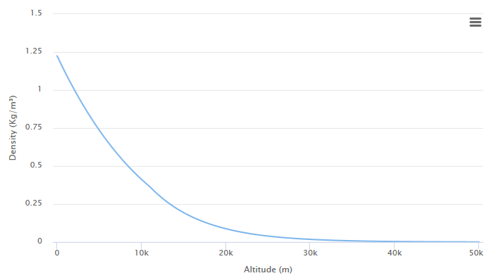
So far, we have not considered the role of the atmospheric density coefficient rho . It is logical that the force of dispersion is proportional to the density of the atmosphere. The more molecules per cubic meter, the greater the probability of photon scattering. The difficulty lies in the fact that the structure of the atmosphere is very complex, it consists of several layers with different pressures, densities and temperatures. Fortunately for us, the bulk of Rayleigh scattering occurs in the first 60 km of the atmosphere. In the troposphere, the temperature decreases linearly, and the pressure decreases exponentially.
The diagram below shows the relationship between density and height in the lower atmosphere.
Value rho left(h right) represents the measurement of the atmosphere at altitude h meters, normalized in such a way that starts from scratch. In many scientific articles r h o also called the density coefficient , because it can also be defined as follows:
r h o l e f t ( h r i g h t ) = f r a c d e n s i t y l e f t ( h r i g h t ) d e n s i t y l e f t ( 0 r i g h t )
Dividing true density by d e n s i t y l e f t ( 0 r i g h t ) we will get that r h o l e f t ( h r i g h t ) at sea level equals one . However, as highlighted above, the calculation d e n s i t y l e f t ( h r i g h t ) far nontrivial. We can approximate it as an exponential curve; some of you might already understand that the density in the lower atmosphere is decreasing exponentially .
If we want to approximate the density coefficient through an exponential curve, then we can do it as follows:
\ rho \ left (h \ right) = exp \ left \ {- \ frac {h} {H} \ right \}
Where H 0 - This is a scale factor called the reduced height . For Rayleigh scattering in the lower layers of the Earth’s atmosphere, it is often considered that H = $ 850 meters (see diagram below). For light scattering by a spherical particle, the value is often approximately equal to 1200 meters.
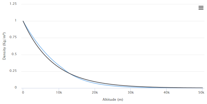
The value used for H does not give the best approximation rho left(h right) . However, this is actually not a problem. Most of the values presented in this tutorial are subject to serious approximations. To create visually pleasing results, it will be much more efficient to adjust the available parameters to reference images.
Exponential decrease
In the previous part of the tutorial, we derived an equation showing us how to take into account the scattering to the outside, to which a ray of light is subjected after interacting with a single particle. The value used to simulate this phenomenon is called the scattering coefficient. beta . To take it into account, we introduced the coefficients beta .
In the case of Rayleigh scattering, we also derived a closed form for calculating the amount of light confirmed by atmospheric scattering in a single interaction:
beta left( lambda,h right)= frac8 pi3 left(n2−1 right)23 frac rho left(h r i g h t ) N f r a c 1 l a m b d a 4
When calculating at sea level, i.e. h=0 The equation gives the following results:
beta left(680nm right)=0.00000519673
beta left(550nm right)=0.0000121427
b e t a l e f t ( 440 n m r i g h t ) = 0.0000296453
Where 680 , 550 and 440 - wavelengths roughly corresponding to red, green, and blue.
What is the meaning of these numbers? They represent the fraction of light that is lost in a single interaction with a particle. Assuming that the beam of light initially has brightness I 0 and passes a segment of the atmosphere with a (total) scattering coefficient b e t a , the amount preserved after the scattering of light is equal to:
I 1 = I 0 ⏟ initial energy - I 0 β ⏟ energy lost = I 0 ( 1 - β )
This is true for a single collision, but we are interested in how much energy is dissipated during a certain distance. This means that the remaining light undergoes this process at every point.
When light passes through a homogeneous medium with a scattering coefficientβhow can we calculate which part of it will remain when moving a certain distance?
For those of you who have studied mathematical analysis, this may seem familiar. When the multiplicative process is repeated on a continuous segment( 1 - β )then the Euler number appears on the scene . The amount of light that persists after passingx meters equals:
I=I0exp{−βx}
And again we are faced with an exponential function. It has nothing to do with the exponential function describing the density coefficient rho .Both phenomena are described by exponential functions because both of them are subject to exponential decrease. In addition, there is no connection between them.
. , , :
I 1 = I 0 ( 1 - β2 )
I 2 = I 1 ( 1 - β2 )
:
I 2 = I 0 ( 1 - β2 )(1-β2 )=
=I0(1−β2)2
I2 . ? ? ? :
I=limn→∞I0(1−βn )n
Where lim n → ∞ — , . , ∞ , - β∞ .
:
lim n → ∞ ( 1 - βn )n=e-β=exp{-β}
, .
Uniform transmission
In the second part of the tutorial, we introduced the concept of transmission Tas a fraction of the light remaining after the scattering process as it passes through the atmosphere. Now we have all the elements to derive the equation describing it.
Let's look at the scheme below and think about how we can calculate the transmittance for the segment¯CP . You can easily see that the rays of light reaching Cpass through the empty space. Therefore, they are not scattered. Therefore, the amount of light inCreally equal to the brightness of the sun IS . During this journey to Ppart of the light is scattered from the path; therefore the amount of light reachingP ( IP ) will be less than IS .
The amount of diffused light depends on the distance traveled. The longer the path, the stronger the attenuation will be. According to the law of exponential decrease, the amount of light at a pointIP can be calculated as follows:
IP=ISexp{−β¯CP}
Where ¯CP - the length of the segment from C before P , but exp{x}- exponential function ex .
Atmospheric transmission
We based our equation on the assumption that the probability of reflection ( the scattering coefficient β same at every point along ¯CP . Unfortunately, this is not the case.
The scattering coefficient strongly depends on the density of the atmosphere. The more air molecules per cubic meter, the higher the probability of a collision. The density of the planet’s atmosphere is not uniform, and varies with altitude. It also means that we cannot calculate outward scattering.¯CPin one step. To solve this problem, we need to calculate the dispersion to the outside at each point using the scattering coefficient.
To understand how this works, let's start with an approximation. Section¯CP divided by two ¯CQ and ¯QP .

First we calculate the amount of light from C which reaches Q :
IQ=ISexp{−β(λ,h0)¯CQ}
Then we use the same approach to calculate the amount of light reaching P of Q :
IP=IQexp{−β(λ,h1)¯QP}
If we substitute IQ in the second equation and simplify, we get:

If a ¯CQ and ¯QP have the same length ds , we can further simplify the expression:
In the case of two segments of the same length with different scattering coefficients outward, it is calculated by summing the scattering coefficients of individual segments and multiplied by the lengths of the segments.
We can repeat this process with an arbitrary number of segments, ever closer to the true value. This will lead us to the following equation:
IP=ISexp{−∑Q∈¯CPβ(λ,hQ)ds}
Where hQ - point height Q .
The method of dividing a line into a set of segments, which we have just used, is called numerical integration .
If we assume that the initial amount of received light is1 , then we obtain the equation of atmospheric transmission through an arbitrary segment:
T(¯CP)=exp{−∑Q∈¯CPβ(λ,hQ)ds}
We can further expand this expression. replacing the totalβ this value used in Rayleigh scattering β :
T(¯CP)=exp{−∑Q∈¯CP8π3(n2−1)23ρ(hQ)N1λ4ds}
Many factors β are constant, so that they can be taken out for the sum:
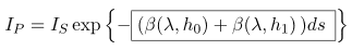
T(¯CP)=exp{−8π3(n2−1)231N1λ4⏟constantβ(λ)optical depthD(¯CP)⏞∑Q∈¯CPρ(hQ)ds}
The amount expressed by summation is called the optical thickness. D(¯CP)which we will calculate in the shader. The remainder is an increment factor that can be calculated only once, and it corresponds to the scattering coefficient at sea level . In the finished shader, we will calculate only the optical thickness, and the scattering coefficients at sea levelβ will pass as input.
Summarize:
T(¯CP)=exp{−β(λ)D(¯CP)}
Part 5. Atmospheric shader.
Introduction
Shader writing
We can start writing a shader for this effect in an infinite number of ways. Since we want to render atmospheric scattering on the planets, it is logical to assume that it will be used on the spheres.
If you use this tutorial to create a game, there is a chance that you will apply a shader to a ready-made planet. Adding atmospheric scatter calculations over the top is possible, but usually gives poor results. The reason is that the atmosphere is larger than the radius of the planet, so it needs to be rendered on a slightly larger transparent sphere. The figure below shows how the atmosphere extends above the surface of the planet, mixing with the empty space behind it.
The application of scattered material to a separate sphere is possible, but redundant. In this tutorial, I suggest expanding Standard Surface Shader Unity by adding a shader pass that renders the atmosphere in a slightly larger sphere. We will call it the atmospheric sphere .
Shader with two passes
If you have previously worked with Unity surface shaders , you might have noticed that they do not support the
Pass block, with which several passes are set in the vertex and fragment shaders .Creating a two-pass shader may be as simple as adding two separate sections of CG code into one
SubShader block: Shader "Custom/NewSurfaceShader" { Properties { _Color ("Color", Color) = (1,1,1,1) _MainTex ("Albedo (RGB)", 2D) = "white" {} _Glossiness ("Smoothness", Range(0,1)) = 0.5 _Metallic ("Metallic", Range(0,1)) = 0.0 } SubShader { // --- --- Tags { "RenderType"="Opaque" } LOD 200 CGPROGRAM // Cg ENDCG // ------------------ // --- --- Tags { "RenderType"="Opaque" } LOD 200 CGPROGRAM // Cg ENDCG // ------------------- } FallBack "Diffuse" } You can change the first pass to render the planet. From now on, we will focus on the second pass, implementing atmospheric scattering in it.
Normal extrusion
The atmospheric sphere is slightly larger than the planet. This means that the second pass must extrude the sphere out. If smooth normals are used in the model you are using, then we can achieve this effect by using a technique called normal extrusion .
Normal extrusion is one of the oldest shader tricks, and is usually one of the first to learn. In my blog there are many references to it; A good start can be a Post A Surface Shader from the A Gentle Introduction to Shaders series.
If you are unfamiliar with how extrusion of normals works, then I will explain: all vertices are processed by the shader using its vertex function . We can use this function to change the position of each vertex, making the sphere larger.
The first step is to change the
pragma directive by adding vertex:vert to it vertex:vert ; this will force Unity to execute the vert function for each vertex. #pragma surface surf StandardScattering vertex:vert void vert (inout appdata_full v, out Input o) { UNITY_INITIALIZE_OUTPUT(Input,o); v.vertex.xyz += v.normal * (_AtmosphereRadius - _PlanetRadius); } This code snippet shows a vertex function extruding a sphere along its normals. The magnitude of the extrusion sphere depends on the size of the atmosphere and the size of the planet. Both of these values need to be passed to the shader as properties that can be accessed through the material inspector .
Our shader also needs to know where the center of the planet is. We can add its calculation to the vertex function too. Finding the center point of an object in the space of the world was discussed in the article Vertex and Fragment Shaders .
struct Input { float2 uv_MainTex; float3 worldPos; // Unity float3 centre; // }; void vert (inout appdata_full v, out Input o) { UNITY_INITIALIZE_OUTPUT(Input,o); v.vertex.xyz += v.normal * (_AtmosphereRadius - _PlanetRadius); o.centre = mul(unity_ObjectToWorld, half4(0,0,0,1)); } UNITY_INITIALIZE_OUTPUT . The shader obtains the position of the vertices in the object space, and it needs to project them into the coordinates of the world using the positions, scale and rotation provided by Unity.And this is one of the operations performed by
UNITY_INITIALIZE_OUTPUT . Without it, we would have to write the code necessary for these calculations ourselves.Additive blending
Another interesting feature that we need to deal with is transparency. Usually transparent material allows you to see what is behind the object. This solution will not work in our case, because the atmosphere is not just a transparent piece of plastic. Light passes through it, so we need to use additive blending mode to increase the luminosity of the planet.
In the default Unity surface shader, no blend mode is enabled by default. To change the situation, we will have to replace the tags in the second pass with the following:
Tags { "RenderType"="Transparent" "Queue"="Transparent"} LOD 200 Cull Back Blend One One The
Blend One One expression is used by the shader to refer to the additive blending mode.Own lighting function
Most often, when writing a surface shader, programmers change its
surf function, which is used to provide “physical” properties, such as albedo, smoothness of the surface, metallic properties, etc. All these properties are then used by the shader to compute realistic shading.In our case, these calculations are not required. To get rid of them, we need to remove the lighting model used by the shader. I examined this topic in detail; You can study the following posts to figure out how to do it:
- 3D Printer Shader Effect ( transfer to Habré)
- CD-ROM Shader: Diffraction Grating
- Fast Subsurface Scattering in Unity ( transfer to Habré)
The new lighting model will be called
StandardScattering ; we must create functions for real-time lighting and global lighting, that is, respectively, LightingStandardScattering and LightingStandardScattering_GI .In the code we need to write, properties such as the direction of light and the direction of view will also be used. They can be obtained using the following code snippet.
#pragma surface surf StandardScattering vertex:vert #include "UnityPBSLighting.cginc" inline fixed4 LightingStandardScattering(SurfaceOutputStandard s, fixed3 viewDir, UnityGI gi) { float3 L = gi.light.dir; float3 V = viewDir; float3 N = s.Normal; float3 S = L; // float3 D = -V; // , ... } void LightingStandardScattering_GI(SurfaceOutputStandard s, UnityGIInput data, inout UnityGI gi) { LightingStandard_GI(s, data, gi); } In
... will be the shader code itself, which is needed to implement this effect.Floating point accuracy
In this tutorial we will assume that all calculations are made in meters. This means that if we need to simulate the Earth, we need a sphere with a radius of 6,371,000 meters. In fact, in Unity, this is not possible due to floating-point number errors that occur when you have to work with very large and very small numbers at the same time.
To circumvent these limitations, you can change the scale of the scattering coefficient to compensate. For example, if a planet has a radius of only 6.371 meters, then the scattering coefficient
beta left( lambda right) should be more than 1,000,000 times, and the height given H - 1,000,000 times smaller.
In my project Unity all properties and calculations are expressed in meters. This allows us to use real, physical values for the scattering coefficients and the reduced height. However, the shader gets the size of the sphere in meters so that it can convert the scale from Unity units to real scale meters.
Part 6. The intersection of the atmosphere.
As stated above, the only way to calculate the optical thickness of a segment passing through the atmosphere is numerical integration . This means that it is necessary to divide the interval into smaller segments of length. ds and calculate the optical thickness of each, considering its density constant.
Image above is optical thickness. overlineAB It is calculated by four samples, each of which takes into account the density in the center of the segment itself.
The first step will obviously be finding the points A and B . If we assume that the objects we are rendering are a sphere, then Unity will try to render its surface. Each pixel on the screen corresponds to a point on the sphere. In the figure below, this point is called O (from origin ). In surface shader O corresponds to the
worldPos variable in the Input structure. This is the amount of work the shader does; the only information available to us is O direction D which denotes the direction of the ray of sight , and the atmospheric sphere centered C and radius R . The difficulty is in calculating A and B . It will be the quickest to use geometry, reducing the task to finding the intersection of the atmospheric sphere and the ray of visibility of the camera.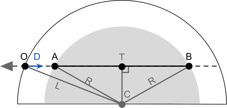
First, it is worth noting that O , A and B lie on the line of sight. This means that we can treat their position not as a point in 3D space, but as distance from the line of sight to origin. A - this is the real point (represented in the shader as
float3 ), and AO - distance to the starting point O (stored as float ). A and AO - two equally correct ways of designating the same point, that is true:A=O+ overlineAOD
B=O+ overlineBOD
where is the entry with the dash above overlineXY denotes the length of the segment between two arbitrary points X and Y .
In the shader code for efficiency we will use AO and BO and calculate them from OT :
overlineAO= overlineOT− overlineAT
overlineBO= overlineOT+ overlineBT
It is also worth noting that the segments overlineAT and overlineBT have the same length. Now, to find the points of intersection, we need to calculate overlineAO and overlineAT .
Section overlineOT it is easiest to calculate. If you look at the diagram above, you can see that overlineOT is a projection of a vector CO on the ray of sight. Mathematically, this projection can be performed using a scalar product . If you are familiar with shaders, you may know that a scalar product is a measure of how “aligned” the two directions are. When it is applied to two vectors, and one of them has a unit length, it becomes the projection operator:
overlineOT= left(C−O right) cdotD
It is also worth noting that
left(C−O right) - this is a three-dimensional vector, and not the length of the segment between C and O .
Next, we need to calculate the length of the segment overlineAT . It can be calculated using the Pythagon theorem in the triangle overset triangleACT . She claims that:
R2= overlineAT2+ overlineCT
And this means that:
overlineAT= sqrtR2− overlineCT
Length overlineCT still unknown. However, it can be calculated by again applying the Pythagorean theorem to the triangle overset triangleOCT :
overlineCO2= overlineOT2+ overlineCT2
overlineCT= sqrt overlineCO2− overlineOT2
Now we have all the necessary quantities. Summarize:
overlineOT= left(C−O right) cdotD
overlineCT= sqrt overlineCO2− overlineOT2
overlineAT= sqrtR2− overlineCT2
overlineAO= overlineOT− overlineAT
overlineBO= overlineOT+ overlineAT
This set of equations has square roots. They are defined only for non-negative numbers. If a R2> overlineCT2 , there is no solution, which means that the ray of visibility does not intersect the sphere.
We can convert this to the following Cg function:
bool rayIntersect ( // Ray float3 O, // Origin float3 D, // // float3 C, // float R, // out float AO, // out float BO // ) { float3 L = C - O; float DT = dot (L, D); float R2 = R * R; float CT2 = dot(L,L) - DT*DT; // if (CT2 > R2) return false; float AT = sqrt(R2 - CT2); float BT = AT; AO = DT - AT; BO = DT + BT; return true; } It returns not one, but three values. overlineAO , overlineBO as well as the binary value of the presence of the intersection. The lengths of these two segments are returned using the out keywords, which save after the completion of the function any changes that it made to these parameters.
Colliding with the planet
There is another problem to consider. Some rays of visibility collide with the planet, so their journey through the atmosphere ends early. One solution is to revise the output above.
A simpler, but less efficient approach is to perform
rayIntersect twice and, if necessary, change the end point.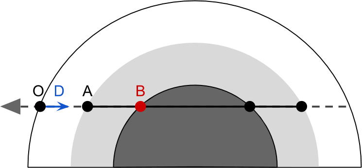
This translates to the following code:
// float tA; // (worldPos + V * tA) float tB; // (worldPos + V * tB) if (!rayIntersect(O, D, _PlanetCentre, _AtmosphereRadius, tA, tB)) return fixed4(0,0,0,0); // // ? float pA, pB; if (rayIntersect(O, D, _PlanetCentre, _PlanetRadius, pA, pB)) tB = pA; Part 7. Atmospheric scatter shader.
In this part, we will finally complete the work on simulating Rayleigh scattering in the atmosphere of the planet.

Sampling ray visibility
Let's recall the atmospheric scattering equation we recently derived:
I=IS sumP in overlineABS left( lambda, theta,h right)T left( overlineCP right)T left( overlinePA right)ds
The amount of light we receive is equal to the amount of light emitted by the sun, IS multiplied by the sum of the individual effects of each point P on the segment overlineAB .
We can implement this function directly in the shader. However, here you need to make some optimization. In the previous part, I said that the expression can be simplified even more. The first thing you can do is to break the scattering function into two main components:
S left( lambda, theta,h right)= beta left( lambda,h right) gamma left( theta right)= beta left( lambda right) rho left(h right) gamma left( theta right)
Phase function gamma left( theta right) and dispersion coefficient at sea level beta left( lambda right) are constants relative to the sum, because the angle theta and wavelength lambda do not depend on the sampled point. Therefore, they can be taken for the amount of:
I=IS beta left( lambda right) gamma left( theta right) sumP in overlineABT left( overlineCP right)T left( overlinePA right) rho left(h right)ds
This new expression is mathematically similar to the previous one, but more efficiently in the calculation, because the most "heavy" parts are derived from the sum.
We are not yet ready for its implementation. There is an infinite number of points P which we must consider. Reasonable approximation I will be splitting overlineAB shorter lengths ds and the addition of the influence of each individual segment. By doing this, we can assume that each segment is small enough to have a constant density. In general, this is not the case, but if ds is small enough, then we can achieve a fairly good approximation.
The number of segments in overlineAB we will call the visibility samples , because all the segments are on the line of sight. In the shader this will be the
_ViewSamples property. Since this is a property, we will be able to access it from the material inspector. This allows us to reduce the accuracy of the shader for its performance.The following code snippet allows you to loop around all segments in the atmosphere.
// // P AB float3 totalViewSamples = 0; float time = tA; float ds = (tB-tA) / (float)(_ViewSamples); for (int i = 0; i < _ViewSamples; i ++) { // // ( ) float3 P = O + D * (time + ds * 0.5); // T(CP) * T(PA) * ρ(h) * ds totalViewSamples += viewSampling(P, ds); time += ds; } // I = I_S * β(λ) * γ(θ) * totalViewSamples float3 I = _SunIntensity * _ScatteringCoefficient * phase * totalViewSamples; The
time variable is used to track how far we are from the starting point. O . After each iteration, it is incremented by ds .Optical thickness PA
Each point on the line of sight overlineAB contributes to the final color of the pixel we draw. This contribution, to put it mathematically, is the value within the sum:
I=IS beta left( lambda right) gamma left( theta right) sumP in overlineAB underset textlightcontributionofL left(P right) underbraceT left( overlineCP right)T left( overlinePA right) rho left(h right)ds
Let's try to simplify this expression, as in the last paragraph. We can further expand the expression above by replacing T by its definition:
T \ left (\ overline {XY} \ right) = \ exp \ left \ {- \ beta \ left (\ lambda \ right) D \ left (\ overline {XY} \ right) \ right \}
The result of passing through overlineCP and overlinepa turns into:
T left( overlineCP right)T left( overlinePA right)=
= \ underset {T \ left (\ overline {CP} \ right)} {\ underbrace {\ exp \ left \ {- \ beta \ left (\ lambda \ right) D \ left (\ overline {CP} \ right ) \ right \}}} \, \ underset {T \ left (\ overline {PA} \ right)} {\ underbrace {\ exp \ left \ {- \ beta \ left (\ lambda \ right) D \ left ( \ overline {PA} \ right) \ right \}}} =
= \ exp \ left \ {- \ beta \ left (\ lambda \ right) \ left (D \ left (\ overline {CP} \ right) + D \ left (\ overline {PA} \ right) \ right) \ right \}
The combined transmittance is modeled as an exponential reduction, whose coefficient is the sum of the optical thickness along the path traveled by the light ( overlineCP and overlinepa ) multiplied by the scattering coefficient at sea level ( beta at h=0 ).
The first quantity we begin to calculate is the optical thickness of the segment. overlinepa which goes from the point of entry into the atmosphere to the point at which we are currently sampling in the for loop. Let's remember the definition of optical thickness:
D \ left (\ overline {PA} \ right) = \ sum_ {Q \ in \ overline {PA}} {\ exp \ left \ {- \ frac {h_Q} {H} \ right \}} \, ds
If we had to implement it "in the forehead", then we would create an
opticalDepth function, which samples the loop between P and A . This is possible, but very inefficient. In fact, D left( overlinePA right) - This is the optical thickness of the segment, which we are already analyzing in the outermost for loop. We can save a lot of calculations if we calculate the optical thickness of the current segment, centered at P ( opticalDepthSegment ), and continue to summarize it in a for loop ( opticalDepthPA ). // float opticalDepthPA = 0; // // P AB float time = tA; float ds = (tB-tA) / (float)(_ViewSamples); for (int i = 0; i < _ViewSamples; i ++) { // // ( ) float3 P = O + D * (time + viewSampleSize*0.5); // // ρ(h) * ds float height = distance(C, P) - _PlanetRadius; float opticalDepthSegment = exp(-height / _ScaleHeight) * ds; // // D(PA) opticalDepthPA += opticalDepthSegment; ... time += ds; } Light sampling
If we return to the expression for the influence of light P , the only required quantity is the optical thickness of the segment. overlineCP ,
L \ left (P \ right) = \ underset {\ text {combined transmittance}} {\ underbrace {\ exp \ left \ {- \ beta \ left (\ lambda \ right) \ left (D \ left (\ overline {CP} \ right) + D \ left (\ overline {PA} \ right) \ right) \ right \}}} \, \ underset {\ text {optical depth of} \, ds} {\ underbrace {\ rho \ left (h \ right) ds}}
We will move the code that calculates the optical thickness of the segment overlineCP into a function called
lightSampling . The name is taken from a ray of light that is a segment starting at P and directed towards the sun. We called the point at which it comes out of the atmosphere C .However, the
lightSampling function lightSampling not simply calculate the optical thickness. overlineCP . So far we have considered only the influence of the atmosphere and ignored the role of the planet itself. Our equations do not take into account the possibility that a ray of light moving from P to the sun, may collide with the planet. If this happens, then all calculations performed up to this point are not applicable, because the light does not actually reach the camera.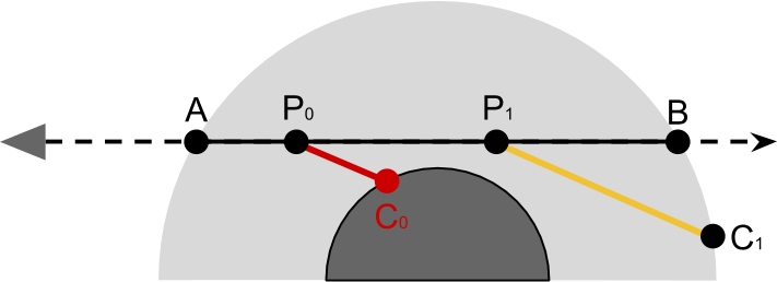
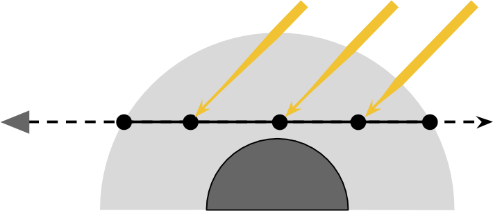
In the diagram below it is easy to see that the effect of light P0 need to be ignored because no sun light reaches P0 . When cyclically moving points between P and C The
lightSampling function also checks if there has been a collision with a planet. This can be done by checking the height of the point for negativity. bool lightSampling ( float3 P, // float3 S, // out float opticalDepthCA ) { float _; // float C; rayInstersect(P, S, _PlanetCentre, _AtmosphereRadius, _, C); // PC float time = 0; float ds = distance(P, P + S * C) / (float)(_LightSamples); for (int i = 0; i < _LightSamples; i ++) { float3 Q = P + S * (time + lightSampleSize*0.5); float height = distance(_PlanetCentre, Q) - _PlanetRadius; // if (height < 0) return false; // opticalDepthCA += exp(-height / _RayScaleHeight) * ds; time += ds; } return true; } The above function first computes a point. Cwith the help of
rayInstersect. Then she divides the segment¯PAinto segments _LightSamplesof length ds. The calculation of the optical thickness is the same as that used in the outermost loop.The function returns false if a collision with a planet has occurred. We can use this to update the missing code of the outermost loop, replacing
.... // D(CP) float opticalDepthCP = 0; bool overground = lightSampling(P, S); if (overground) { // // T(CP) * T(PA) = T(CPA) = exp{ -β(λ) [D(CP) + D(PA)]} float transmittance = exp ( -_ScatteringCoefficient * (opticalDepthCP + opticalDepthPA) ); // // T(CPA) * ρ(h) * ds totalViewSamples += transmittance * opticalDepthSegment; } Now that we have considered all the elements, our shader is ready.
[Approx. Trans .: on the Patreon author's page you can buy access to the Standard and Premium versions of the finished shader.]
Source: https://habr.com/ru/post/345630/
All Articles