Deep neural networks are now a trendy topic.

There are a lot of tutorials and video lectures on the web, and other materials discussing the basic principles of building neural networks, their architecture, learning strategies, etc. Traditionally, neural networks are trained by displaying a neural network of image packets from a training sample and correcting the coefficients of this network using the back propagation error method . One of the most popular tools for working with neural networks is Google's Tensorflow library.

The neural network in Tensorflow is represented by a sequence of layer operations.
(such as matrix multiplication, convolution , pooling, etc.). The layers of the neural network, together with the operations of adjusting the coefficients, form a calculation graph.

The learning process of the neural network in this case consists in the "presentation" of the neural
networks of object packages, comparing predicted classes with true ones, calculations
errors and modifications of neural network coefficients.

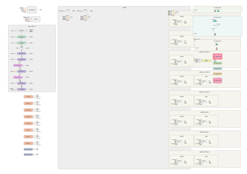
In this case, Tensoflow hides the technical details of the training and the implementation of the coefficient adjustment algorithm, and from the programmer's point of view, one can speak mostly only about the computation graph, which produces “predictions”. Compare the computation graph that the programmer thinks about.

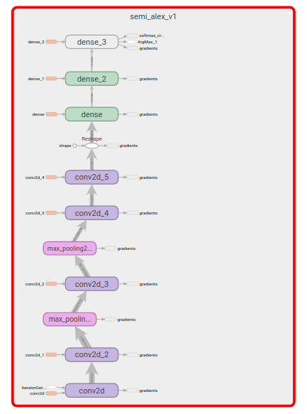
with the graph which, among other things, performs the adjustment of coefficients

.

But what Tensorflow cannot do for a programmer is to convert the input dataset into a convenient for training neural network. Although the library has quite a few "basic blocks".

How to use them to build an effective conveyor for the "power" ( feed ) neural network input data and I want to tell in this article.

As an example of the problem, ImageNet datasset will be used, which was recently published as a competition for detecting objects on Kaggle. We will train the network to detect one object, the one with the largest bounding box.

If you have not tried to work with this library, it may be worth exploring the basic concepts, for example, in the Tensorflow deep learning library article, or on the official website.

Preparatory steps

The following assumes that you have

• [Python] [python_org] is installed, the examples use Python 2.7,
  but there should be no difficulty in porting them to Python 3. *
• library [Tensorflow and Python interface to it] [install_tensorflow]
• downloaded and unpacked [dataset] [download_dataset] from Kaggle competition

Traditional library aliases:

import tensorflow as tf import numpy as np 

Data preprocessing

To load data, we will use the mechanisms provided by the module for working with datasets in Tensorflow.

For training and validation, we need a dataset, in which both images and their descriptions are at the same time. But in the downloaded dataset files with images and annotations are neatly laid out in different daddies.

Therefore, we will make an iterator that is iterated over the corresponding pairs.

 ANNOTATION_DIR = os.path.join("Annotations", "DET") IMAGES_DIR = os.path.join("Data", "DET") IMAGES_EXT = "JPEG" def image_annotation_iterator(dataset_path, subset="train"): """ Yields tuples of image filename and corresponding annotation. :param dataset_path: Path to the root of uncompressed ImageNet dataset :param subset: one of 'train', 'val', 'test' :return: iterator """ annotations_root = os.path.join(dataset_path, ANNOTATION_DIR, subset) print annotations_root images_root = os.path.join(dataset_path, IMAGES_DIR, subset) print images_root for dir_path, _, file_names in os.walk(annotations_root): for annotation_file in file_names: path = os.path.join(dir_path, annotation_file) relpath = os.path.relpath(path, annotations_root) img_path = os.path.join( images_root, os.path.splitext(relpath)[0] + '.' + IMAGES_EXT ) assert os.path.isfile(img_path), \ RuntimeError("File {} doesn't exist".format(img_path)) yield img_path, path 

From this, you can already make a dataset and run "processing on the graph",
for example, retrieve file names from dataset.
We create:

 files_dataset = tf.data.Dataset.from_generator( functools.partial(image_annotation_iterator, "./ILSVRC"), output_types=(tf.string, tf.string), output_shapes=(tf.TensorShape([]), tf.TensorShape([])) ) 

To extract data from dataset, we need an iterator
make_one_shot_iterator will create an iterator that passes through
given once. Iterator.get_next() creates a tensor in which to load
data from the iterator.

 iterator = files_dataset.make_one_shot_iterator() next_elem = iterator.get_next() 

Now you can create a session and "calculate the values" of the tensor:

 with tf.Session() as sess: for i in range(10): element = sess.run(next_elem) print i, element 

But for use in neural networks, we need not file names, but images in the form of "three-layer" matrices of the same form and the category of these images in the form of "one hot" vector

We encode categories of images

Parsing annotation files is not very interesting by itself. I used the BeautifulSoup package for this. Annotation helper class can initialize from the file path and store a list of objects. First we need to compile a list of categories in order to know the size of the vector for encoding cat_max . And also make the display of string categories in the number of [0..cat_max] . The creation of such mappings is also not very interesting, we will further assume that the cat2id and id2cat contain the forward and reverse mapping described above.

The function of converting a file name into a coded category vector.

You can see that another category is added for the background: in some images no objects are marked.

 def ann_file2one_hot(ann_file): annotation = reader.Annotation("unused", ann_file) category = annotation.main_object().cls result = np.zeros(len(cat2id) + 1) result[cat2id.get(category, len(cat2id))] = 1 return result 

Apply the transformation to dataset:

 dataset = file_dataset.map( lambda img_file_tensor, ann_file_tensor: (img_file_tensor, tf.py_func(ann_file2one_hot, [ann_file_tensor], tf.float64)) ) 

The map method returns a new dataset, in which a function is applied to each line of the initial dataset. The function does not actually apply until we started to iterate over the resulting dataset.

You can also notice that we wrapped our function in tf.py_func . as parameters, the tensors are included in the transformation function, and not the values ​​that lie in them.

And to work with strings, this wrapper is needed.

Upload an image

In Tensorflow there is a rich library for working with images . Use it to download them. We need to: read the file, decode it into a matrix, bring the matrix to a standard size (for example, the average), normalize the values ​​in this matrix.

 def image_parser(file_name): image_data = tf.read_file(file_name) image_parsed = tf.image.decode_jpeg(image_data, channels=3) image_parsed = tf.image.resize_image_with_crop_or_pad(image_parsed, 482, 415) image_parsed = tf.cast(image_parsed, dtype=tf.float16) image_parsed = tf.image.per_image_standardization(image_parsed) return image_parsed 

Unlike the previous function, here the file_name is a tensor, which means we don’t need to wrap this function, we will add it to the previous snippet:

 dataset = file_dataset.map( lambda img_file_tensor, ann_file_tensor: ( image_parser(img_file_tensor), tf.py_func(ann_file2one_hot, [ann_file_tensor], tf.float64) ) ) 

Let's check that our graph of graphs produces something meaningful:

  iterator = dataset.make_one_shot_iterator() next_elem = iterator.get_next() print type(next_elem[0]) with tf.Session() as sess: for i in range(3): element = sess.run(next_elem) print i, element[0].shape, element[1].shape 

It should work:

 0 (482, 415, 3) (201,) 1 (482, 415, 3) (201,) 2 (482, 415, 3) (201,) 

As a rule, at the very beginning it would be necessary to divide the dataset into 2 or 3 parts for training / validation / testing. We will use the division for training and validation from the downloaded archive.

Designing a Calculation Graph

We will train a convolutional neural network (English convolutional neural netwrok, CNN) by a method similar to a stochastic gradient descent , but we will use its improved version of Adam . To do this, we need to combine our instances into "packages" (eng. Batch). In addition, to utilize multiprocessing (and, at best, the availability of a GPU for training), you can enable background data paging

 BATCH_SIZE = 16 dataset = dataset.batch(BATCH_SIZE) dataset = dataset.prefetch(2) 

We will combine the packages on BATCH_SIZE instances and pump up 2 such packages.

During training, we want to periodically drive validation, on a sample that does not participate in training. So we need to repeat all the manipulations above for another dataset.

Fortunately, all of them can be combined into a function such as dataset_from_file_iterator and create two datasets:

 train_dataset = dataset_from_file_iterator( functools.partial(image_annotation_iterator, "./ILSVRC", subset="train"), cat2id, BATCH_SIZE ) valid_dataset = ... #     subset="val" 

But since we want to continue using the same graph of calculations for training and validation, we will create a more flexible iterator. That which allows him to reinitialize.

  iterator = tf.data.Iterator.from_structure( train_dataset.output_types, train_dataset.output_shapes ) train_initializer_op = iterator.make_initializer(train_dataset) valid_initializer_op = iterator.make_initializer(valid_dataset) 

Later, after performing this or that operation, we can switch the iterator from one dataset to
other.

 with tf.Session(config=config, graph=graph) as sess: sess.run(train_initialize_op) #  # ... sess.run(valid_initialize_op) #  # ... 

For teprey we need to describe our neural network, but we will not go into this question.
We assume that the semi_alex_net_v1(mages_batch, num_labels) function semi_alex_net_v1(mages_batch, num_labels) builds the desired architecture and returns a tensor with output values ​​predicted by the neural network.

Let us set the error function, and subtleties, the optimization operation:

 img_batch, label_batch = iterator.get_next() logits = semi_alexnet_v1.semi_alexnet_v1(img_batch, len(cat2id)) loss = tf.losses.softmax_cross_entropy( logits=logits, onehot_labels=label_batch) labels = tf.argmax(label_batch, axis=1) predictions = tf.argmax(logits, axis=1) correct_predictions = tf.reduce_sum(tf.to_float(tf.equal(labels, predictions))) optimizer = tf.train.AdamOptimizer().minimize(loss) 

Training and validation cycle

Now you can start learning:

 with tf.Session() as sess: sess.run(tf.local_variables_initializer()) sess.run(tf.global_variables_initializer()) sess.run(train_initializer_op) counter = tqdm() total = 0. correct = 0. try: while True: opt, l, correct_batch = sess.run([optimizer, loss, correct_predictions]) total += BATCH_SIZE correct += correct_batch counter.set_postfix({ "loss": "{:.6}".format(l), "accuracy": correct/total }) counter.update(BATCH_SIZE) except tf.errors.OutOfRangeError: print "Finished training" 

Above, we create a session, initialize global and local variables in the graph, initialize the iterator with training data. [tqdm] [tgdm] does not apply to the learning process, it is simply a convenient tool for visualizing progress.

In the context of the same session, we launch and validation: the validation cycle looks very similar. The main difference: the optimization operation does not start.

 with tf.Session() as sess: # Train # ... # Validate counter = tqdm() sess.run(valid_initializer_op) total = 0. correct = 0. try: while True: l, correct_batch = sess.run([loss, correct_predictions]) total += BATCH_SIZE correct += correct_batch counter.set_postfix({ "loss": "{:.6}".format(l), "valid accuracy": correct/total }) counter.update(BATCH_SIZE) except tf.errors.OutOfRangeError: print "Finished validation" 

Epochs and Checkpoints

One simple pass through all the images is certainly not enough for training. And you need the code for training and validation above to perform in a loop (within one session).

Perform either a fixed number of iterations, or until training helps. A single pass through the entire data set is traditionally called an epoch (eng. Epoch).

In case of unforeseen stops of training and for further use of the model, you need to save it. To do this, when creating an execution graph, you need to create a Saver class object. And in the course of training to maintain the state of the model.

 #   # ... saver = tf.train.Saver() #   with tf.Session() as sess: for i in range(EPOCHS): # Train # ... # Validate # ... saver.save(sess, "checkpoint/name") 

What's next

We learned how to create datasets, transform them using functions of working with
tensors, as well as the usual functions written in python. We learned how to load images in the background loop without trying to load them into memory or save them in the decompressed form. They also learned to save the trained model.

By applying part of the steps described above and downloading it, you can make a program that will recognize images.

The article does not completely reveal the topics of neural networks as such, their architecture and methods of training. For those who want to figure it out, I can recommend the Deep Learning by Google course on Udacity, it is suitable for beginners as well, without a serious background. About the use of convolutional neural networks for recognition there is an excellent course of lectures by Convolutional Neural Networks for Visual Recognition from Stanford University. It is also worth looking at coursera ning coursera courses on the Sourcesera. There are also quite a lot of materials on Habrahabr, for example, a good overview of the Tensorflow library from Open Data Science.

UPD: Script and helper libraries are available on Github