Linear Regression with Go

For a long time I was interested in the topic of machine learning. I wondered how machines could learn and predict without any programming - amazing! I was always fascinated by this, but I never studied the topic in detail. Time is a scarce resource, and every time I tried to read about machine learning, I was flooded with information. Mastering all of this seemed difficult and time consuming. I also convinced myself that I did not have the necessary mathematical knowledge even to begin to delve into machine learning.

But in the end I decided to approach this differently. Little by little, I will try to recreate different concepts in the code, starting with the basics and gradually moving to more complex ones, trying to cover as many basic things as possible. I chose Go as the language, this is one of my favorite languages, and besides, I am not familiar with machine learning languages ​​like R or Python.

Getting started

Let's start by creating a simple model to understand what stages the main learning process is.

Suppose you need to forecast house prices in King County, Washington.

First you need to find datasets with real statistics. Based on it, we will create a model.

Let's use dataset with kaggle .

It comes in the form of a csv-file with the following structure:

kc_house_data.csv

id,date,price,bedrooms,bathrooms,sqft_living,sqft_lot,floors,waterfront,view,condition,grade,sqft_above,sqft_basement,yr_built,yr_renovated,zipcode,lat,long,sqft_living15,sqft_lot15 "7129300520","20141013T000000",221900,3,1,1180,5650,"1",0,0,3,7,1180,0,1955,0,"98178",47.5112,-122.257,1340,5650 "6414100192","20141209T000000",538000,3,2.25,2570,7242,"2",0,0,3,7,2170,400,1951,1991,"98125",47.721,-122.319,1690,7639 "5631500400","20150225T000000",180000,2,1,770,10000,"1",0,0,3,6,770,0,1933,0,"98028",47.7379,-122.233,2720,8062 

Inside the file there is everything you need. Each row contains a lot of information, and you have to figure out what exactly will help us to predict prices for houses.
We need:

1. Choose a model.
2. Understand the data.
3. Prepare data for work.
4. To train a model.
5. Test the model.
6. Visualize the model.

1. Model selection

Let's use one of the simplest popular models - linear regression .

This model underlies many others, and it’s good to start a new data analysis with it. If the resulting model will predict well enough, then you will not have to move to a more complex one.

Let's take a closer look at linear regression:

This graph shows the relationship between the two variables.

The vertical axis (Y) reflects the dependent variable — in our case, house prices. The horizontal axis (X) reflects the so-called independent variable - in our case it can be any other data from the dataset, for example, bedrooms, bathrooms, sqft_living ...

Circles in the graph are the y-values for a given x-value (y depends on x ). Red line - linear regression. This line goes through all the values ​​and can be used to predict the possible values ​​of y for a given x .

Our goal is to train the model to build the red line for our task.

Recall that a linear function has the form y = ax + b . We need to find her. More precisely, we need to find values a and b that best suit our data.

2. We understand the data

We know which model we need and which approach we will use. It remains to analyze the data and understand whether they are suitable for our task.

Data for the linear regression model should be normally distributed . That is, the data histogram should be in the form of a bell.

Let's build a graph based on our data and see if they are properly distributed. For this we finally write the code!

Useful packages:

• The encoding / csv from the standard library will help us load dataset and parse its contents.
• github.com/gonum/plot helps build a graph.

This code opens our CSV and draws histograms for all columns, except for ID and Date. So we can choose which columns to use to train the model:

  // we open the csv file from the disk f, err := os.Open("./datasets/kc_house_data.csv") if err != nil { log.Fatal(err) } defer f.Close() // we create a new csv reader specifying // the number of columns it has salesData := csv.NewReader(f) salesData.FieldsPerRecord = 21 // we read all the records records, err := salesData.ReadAll() if err != nil { log.Fatal(err) } // by slicing the records we skip the header records = records[1:] // we iterate over all the records // and keep track of all the gathered values // for each column columnsValues := map[int]plotter.Values{} for i, record := range records { // we want one histogram per column, // so we will iterate over all the columns we have // and gather the date for each in a separate value set // in columnsValues // we are skipping the ID column and the Date, // so we start on index 2 for c := 2; c < salesData.FieldsPerRecord; c++ { if _, found := columnsValues[c]; !found { columnsValues[c] = make(plotter.Values, len(records)) } // we parse each close value and add it to our set floatVal, err := strconv.ParseFloat(record[c], 64) if err != nil { log.Fatal(err) } columnsValues[c][i] = floatVal } } // once we have all the data, we draw each graph for c, values := range columnsValues { // create a new plot p, err := plot.New() if err != nil { log.Fatal(err) } p.Title.Text = fmt.Sprintf("Histogram of %s", records[0][c]) // create a new normalized histogram // and add it to the plot h, err := plotter.NewHist(values, 16) if err != nil { log.Fatal(err) } h.Normalize(1) p.Add(h) // save the plot to a PNG file. if err := p.Save( 10*vg.Centimeter, 10*vg.Centimeter, fmt.Sprintf("./graphs/%s_hist.png", records[0][c]), ); err != nil { log.Fatal(err) } } 

This code generates a set of graphs. Of these, you need to choose one that best meets the conditions of a normal distribution (bell-shaped curve).

Here is the graph I chose ( all histograms ):

This is the graph for the Grade column It is not perfect in terms of normal distribution, but for now this is enough. If you look at all the histograms, you will find a few more that can also be used. If the resulting model is poorly predicted, then we choose another dataset column as a basis.

If that: Grad is an assessment of the quality level of a building. You can read more about the quality levels of buildings here , in the BUILDING GRADE section.

3. Prepare the data

So, for training the model we will use the downloaded dataset. But how do you know if our model is accurate enough?

Let's test it , and for this we will use the same dataset. In order for one dataset to be useful for teaching and testing, we divide it into two parts: one for training, the second for testing. This is a normal approach.

We will train on 80% of the data, and take the remaining 20% ​​for the test. There are other established relationships, but to select the appropriate option, you will most likely have to act by trial and error.

We need to find a balance between the adequacy of data for correct training and testing, so as not to retrain the model.

  // we open the csv file from the disk f, err := os.Open("./datasets/kc_house_data.csv") if err != nil { log.Fatal(err) } defer f.Close() // we create a new csv reader specifying // the number of columns it has salesData := csv.NewReader(f) salesData.FieldsPerRecord = 21 // we read all the records records, err := salesData.ReadAll() if err != nil { log.Fatal(err) } // save the header header := records[0] // we have to shuffle the dataset before splitting // to avoid having ordered data // if the data is ordered, the data in the train set // and the one in the test set, can have different // behavior shuffled := make([][]string, len(records)-1) perm := rand.Perm(len(records) - 1) for i, v := range perm { shuffled[v] = records[i+1] } // split the training set trainingIdx := (len(shuffled)) * 4 / 5 trainingSet := shuffled[1 : trainingIdx+1] // split the testing set testingSet := shuffled[trainingIdx+1:] // we write the splitted sets in separate files sets := map[string][][]string{ "./datasets/training.csv": trainingSet, "./datasets/testing.csv": testingSet, } for fn, dataset := range sets { f, err := os.Create(fn) if err != nil { log.Fatal(err) } defer f.Close() out := csv.NewWriter(f) if err := out.Write(header); err != nil { log.Fatal(err) } if err := out.WriteAll(dataset); err != nil { log.Fatal(err) } out.Flush() } 

The code above generates two files:

• training.csv - contains entries for training the model.
• testing.csv - contains entries for testing.

4. We train model

Now we will start learning. Different packages are suitable for this, we will take github.com/sajari/regression , everything necessary is implemented in it.

Of course, you can write everything from scratch, but for now let's not complicate things.

First, download the records from training.csv , go through them and put in the model data from the columns Price and Grade .

Now we will train the model to find our linear function.

This will deal with the code :

  // we open the csv file from the disk f, err := os.Open("./datasets/training.csv") if err != nil { log.Fatal(err) } defer f.Close() // we create a new csv reader specifying // the number of columns it has salesData := csv.NewReader(f) salesData.FieldsPerRecord = 21 // we read all the records records, err := salesData.ReadAll() if err != nil { log.Fatal(err) } // In this case we are going to try and model our house price (y) // by the grade feature. var r regression.Regression r.SetObserved("Price") r.SetVar(0, "Grade") // Loop of records in the CSV, adding the training data to the regression value. for i, record := range records { // Skip the header. if i == 0 { continue } // Parse the house price, "y". price, err := strconv.ParseFloat(records[i][2], 64) if err != nil { log.Fatal(err) } // Parse the grade value. grade, err := strconv.ParseFloat(record[11], 64) if err != nil { log.Fatal(err) } // Add these points to the regression value. r.Train(regression.DataPoint(price, []float64{grade})) } // Train/fit the regression model. r.Run() // Output the trained model parameters. fmt.Printf("\nRegression Formula:\n%v\n\n", r.Formula) 

After completing the execution, we get the formula:

 Regression Formula: Predicted = -1065201.67 + Grade*209786.29 

5. Testing the model

It is assumed that the generated formula allows you to predict sales prices based on the column Grade.

Test the formula. To do this, we take the testing.csv file created earlier.

Although we have test data, we still need some data on the output, by which we understand how accurate the formula is. For this we use the value of the coefficient of determination .

The coefficient of determination tells us at what proportion of dependent variables we can predict independent variables. In our case - how much house prices can be predicted based on data from the Grade column.

The generated value of the coefficient will be in the range from 0 to 1 (the higher the better).

Here is the code that generates the coefficient of determination:

 func main() { // we open the csv file from the disk f, err := os.Open("./datasets/testing.csv") if err != nil { log.Fatal(err) } defer f.Close() // we create a new csv reader specifying // the number of columns it has salesData := csv.NewReader(f) salesData.FieldsPerRecord = 21 // we read all the records records, err := salesData.ReadAll() if err != nil { log.Fatal(err) } // by slicing the records we skip the header records = records[1:] // Loop over the test data predicting y observed := make([]float64, len(records)) predicted := make([]float64, len(records)) var sumObserved float64 for i, record := range records { // Parse the house price, "y". price, err := strconv.ParseFloat(records[i][2], 64) if err != nil { log.Fatal(err) } observed[i] = price sumObserved += price // Parse the grade value. grade, err := strconv.ParseFloat(record[11], 64) if err != nil { log.Fatal(err) } // Predict y with our trained model. predicted[i] = predict(grade) } mean := sumObserved / float64(len(observed)) var observedCoefficient, predictedCoefficient float64 for i := 0; i < len(observed); i++ { observedCoefficient += math.Pow((observed[i] - mean), 2) predictedCoefficient += math.Pow((predicted[i] - mean), 2) } rsquared := predictedCoefficient / observedCoefficient // Output the R-squared to standard out. fmt.Printf("R-squared = %0.2f\n\n", rsquared) } func predict(grade float64) float64 { return -1065201.67 + grade*209786.29 } 

Please note that the predict function is a linear equation that we generated using a test dataset.

Here's what we got:

 R-squared = 0.46 

Not ideal.

Let's try to visualize our regression and try to improve it.

6. Visualize the model.

For visualization, we will write some more code :

  // we open the csv file from the disk f, err := os.Open("kc_house_data.csv") if err != nil { log.Fatal(err) } defer f.Close() df := dataframe.ReadCSV(f) // pts will hold the values for plotting. pts := make(plotter.XYs, df.Nrow()) // ptsPred will hold the predicted values for plotting. ptsPred := make(plotter.XYs, df.Nrow()) yVals := df.Col("price").Float() for i, floatVal := range df.Col("grade").Float() { pts[i].X = floatVal pts[i].Y = yVals[i] ptsPred[i].X = floatVal ptsPred[i].Y = predict(floatVal) } // Create the plot. p, err := plot.New() if err != nil { log.Fatal(err) } pXLabel.Text = "grade" pYLabel.Text = "house price" p.Add(plotter.NewGrid()) // Add the scatter plot points for the observations. s, err := plotter.NewScatter(pts) if err != nil { log.Fatal(err) } s.GlyphStyle.Radius = vg.Points(2) s.GlyphStyle.Color = color.RGBA{R: 0, G: 0, B: 255, A: 255} // Add the line plot points for the predictions. l, err := plotter.NewLine(ptsPred) if err != nil { log.Fatal(err) } l.LineStyle.Width = vg.Points(0.5) l.LineStyle.Dashes = []vg.Length{vg.Points(2), vg.Points(2)} l.LineStyle.Color = color.RGBA{R: 255, G: 0, B: 0, A: 255} // Save the plot to a PNG file. p.Add(s, l) if err := p.Save(10*vg.Centimeter, 10*vg.Centimeter, "./graphs/first_regression.png"); err != nil { log.Fatal(err) } 

Finally, we got our first linear regression:

If you look closely, it will become clear that the blue circles best fit on a curved line, rather than a straight line.

To improve the result, you can try to replace the current linear parabolic formula: y = ax + bx^2 + c .

And again, use the Grade column to represent the x-variable , and the new formula will look like this:

 price = a * grade + b * grade^2 + c 

Update the code of the training function:

  // ... everything is the same up to here r.SetVar(1, "Grade2") // now we add one more variable, Grade^2 // ... everything is the same also here // except we are now addin the new variable r.Train(regression.DataPoint(price, []float64{grade, math.Pow(grade, 2)})) // ... 

Get a new formula:

 Regression Formula: Predicted = 1639674.31 + Grade*-473161.41 + Grade2*42070.46 

Now you can again calculate the coefficient of determination :

 R-squared = 0.52 

It got better! Remember, you need to get the value as close as possible to 1.

Now update the chart drawing code :

  // ... we open the file etc // pts will hold the values for plotting. pts := make(plotter.XYs, df.Nrow()) yVals := df.Col("price").Float() for i, floatVal := range df.Col("grade").Float() { pts[i].X = floatVal pts[i].Y = yVals[i] } // Create the plot. p, err := plot.New() if err != nil { log.Fatal(err) } pXLabel.Text = "grade" pYLabel.Text = "house price" p.Add(plotter.NewGrid()) // Add the scatter plot points for the observations. s, err := plotter.NewScatter(pts) if err != nil { log.Fatal(err) } s.GlyphStyle.Radius = vg.Points(2) s.GlyphStyle.Color = color.RGBA{R: 0, G: 0, B: 255, A: 255} curve := plotter.NewFunction(predict) curve.LineStyle.Width = vg.Points(3) curve.LineStyle.Dashes = []vg.Length{vg.Points(3), vg.Points(3)} curve.LineStyle.Color = color.RGBA{R: 255, G: 0, B: 0, A: 255} // Save the plot to a PNG file. p.Add(s, curve) if err := p.Save(10*vg.Centimeter, 10*vg.Centimeter, "./graphs/second_regression.png"); err != nil { log.Fatal(err) } 

Updated schedule:

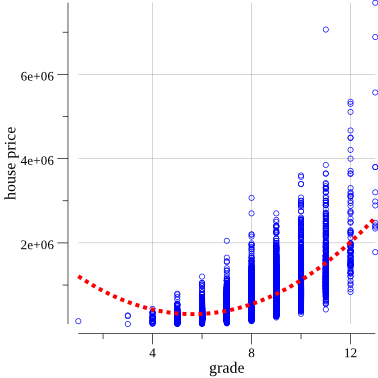
It turned out better.

You can make a number of improvements to get the value of the coefficient of determination closer to 1, if you want - experiment. You can also try to improve the model by changing or combining different variables.

Let's say we are satisfied with the prediction formula, let's start using it. Let's say we want to find out how much money you can earn on selling a house in the Grade 3 category in King County. Insert the Grade value into the formula and get the price:

 598824.2200000001 USD 

I hope you found this introduction to using the linear regression model and Go packages helpful, and you can now begin to learn machine learning.

All code from the article is in the repository .