Monte Carlo option premium calculation vs Black-Scholes formula
The issue is formulated in the previous article .
Namely: how to assess the impact of a certain assumption of the Black-Scholes model on the estimated premium for the European option? Assumptions that the price of the asset being traded has a lognormal distribution. As an alternative to calculating using the Black-Scholes formula, I used the approach of predicting payments to an option buyer using the Monte Carlo method. At the entrance of the program, I filed:
In each case, I calculated the option premium using the formula B-SH and the Monte-Carlo method. I compared the results and made (?) Conclusions:
')

Earlier, I built two hypothetical price series in MS Excel: ABS / USD - a price series described by a lognormal distribution law. And the WRD / USD series is a price series, the distribution of which is characterized by a greater probability of smaller changes with a significant probability of large (> 3σ) changes.
The coefficients in the Excel spreadsheet were selected so that both of these virtual price assets were characterized by the same HV value. Under such conditions and equal options of the option contract (current price, strike, expiration), the premium calculation for the ABS / USD option and WRD / USD according to the Black-Scholes formula will give the same value for both assets.
An alternative way to estimate the size of the premium is to simulate option payouts using the Monte Carlo method. To carry out a series of iterations, at each iteration modeling the price for N days in advance. At the end of the iteration, calculate the option buyer's profit.
The “fair” premium on the option contract will be received by us as the sum of payments divided by the number of iterations. The question is: will the premium calculated in this way (programmatically) coincide with the premium calculated by the formula BS?
And finally, I am going to apply the same methodology for estimating the premium for historical data of real exchange-based assets. Multiple currencies and cryptocurrencies traded for other currencies and cryptocurrencies.
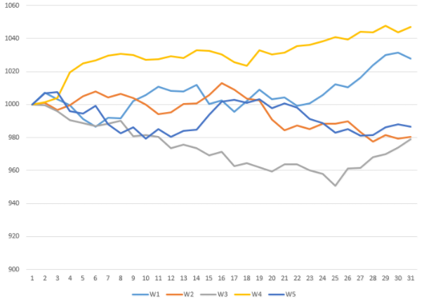
In the following table, I calculated the price of WRD / USD (the price distribution has “thick tails”) several times in a row for 30 days in advance. As before, the price of WRD / USD changed every day in e∆ time.
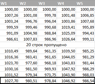
In 2 cases out of 5, the price of an asset WRD / USD increased, in 3 cases it fell:
Accordingly, in 2 cases, the CALL-option buyer was able to realize a profit equal to
(1027.70 - 1000) + (1046.92 - 1000) = $ 74.62.
We divide $ 74.62 by the number of possible outcomes (5) and we get a bonus, which is $ 14.92. Somewhat more than the previous calculation given by the B-Sh method. But so and our method is not very accurate: only 5 iterations.
At this stage, Excel is not enough for us. I conducted 5 simulation experiments: I filled out 5 columns of the price generated for our hypothetical WRD / USD asset. But for our goal - the good convergence of the option premium estimate - 500 experiments are not enough.
In addition, as we remember, the price of WRD / USD is a function of the CB with the density function — the sum of the density functions of two normal distributions. A random sequence obeying the distribution law, which I used as an example. With parameters chosen solely for the purpose of demonstration, but not reflecting the price dynamics of any real product. This is not at all what we need to analyze an exchange asset. We need a program that implements the logic of the form:
The logic of the program at a high level:
In the simple algorithm above, one clause requires an explanation: “preliminary processing of price data”. Let me explain with an example of the price chart for the ABS / USD asset (price distribution is lognormal), which we obtained earlier:
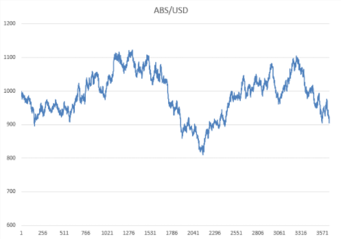
The final price of the ABS / USD asset is lower than the original price. The downtrend of our asset is not a pattern, but the influence of a non-deterministic factor - let me remind you that we used a random number generator.
At the same time, it is known a priori about the ABS / USD asset that its price, in general, drifts equally up or down. That is, in the model, the mathematical expectation of the ABS / USD price deviation is 0.
In the statistical evaluation, the mathematical expectation — the average value of the price change — turned out to be negative.
Is it correct to use for the calculations data that already contain a priori “knowledge” about the negative profitability of an asset? The word "knowledge" is not without reason put in quotes: we know that the ABS / USD asset is equally likely to grow in price and become cheaper. This is the data model we used in the calculation.
On the other hand, statistics show us a negative expectation of daily price dynamics. And this “knowledge” obtained on, in fact, a random sample, we will lay in the model.
ABS / USD is a hypothetical asset. It is definitely possible to say that, for the construction of the table - the distribution function, which will later be used to generate price forecasts, the current trend is a statistical error that needs to be eliminated.
But what if we analyze a real market asset? Not ABS / USD, but, for example, EUR / USD? How to deal with the trend that took place in reality?
My opinion: trend should be removed from price history. The opposite is true if we have "reliable" evidence that the price of an asset will continue to decline in the future. Yes, there are such currencies, goods and other objects of trade, on the dynamics of pricing which economic analysis gives a certain forecast. What can not be said, for example, about the majority of cryptocurrencies.
Where there are enough reasoned statements both in favor of the uptrend and in favor of the downtrend, the historical prices should be “aligned”:
In the figure, the original blue curve was adjusted: a value equal to i * d was subtracted from each i-th price value, where d is equal to the difference between the first and last prices divided by the number of time periods (the number of prices minus 1).
In an application program designed to estimate the value of the premium on an option contract, it is probably worthwhile to provide two calculation options: with the removal of the trend and with the data taken and used as is.
Certainly, where we do not have full confidence in the price dynamics for the forecast period, the trend should be eliminated. And if there is confidence - is it worth spending time studying derivatives, when you can just enter the market with all the available funds and, with a tangible profit, monetize your forecasts?
Another note: the trend does not necessarily eliminate directly from the prices. For example, bitcoin with its growth of more than one hundred percent in one year only after the removal of the trend component from prices will generally go into the negative half-plane along the price axis. The negative price is definitely not suitable for further calculations. The alternative I use is to remove the trend from a range of price changes - ln( fracxixi−1) where xiandxi−1xi - current and previous price values.
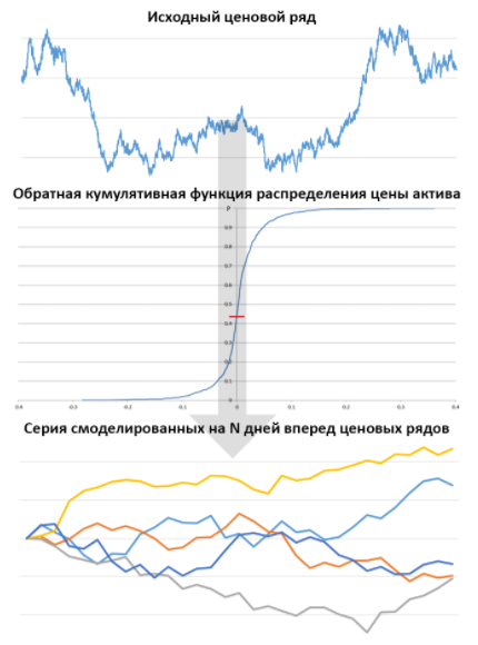
In the program that I bring in the depository of the github code by reference , perhaps the most “intelligent” part is the construction of the inverse cumulative (integral) distribution function and using it to generate a random price increment. The whole process is divided into several steps.
In the first step I get from the prices x1,x2,...,xN increments d1,d2,...,dN−1:di=ln( fracxixi−1)
Further, if the option to eliminate the trend is selected, I get a new series of price increments, subtracting from each value di equal to fracdN−1−d1N−2 .
I sort the price increment values in ascending order.
The process of constructing the inverse distribution function is implemented in one cycle. Imagine that the price changes ( xi+1=xi∗edi a) on discrete values di . What is the probability that the price will change in ed1 or less times where d1 - the smallest of the price increment values in our sample? Obviously, this probability will be frac1N−1 . What is the probability that the price will change in ed2 or less times? Obviously, this probability is equal to the sum of the probabilities of two unrelated outcomes: price changes in ed1 times either in ed2 times or frac1+1N−1 .
Ie, having a sorted row d1,d2,...,dN−1 , it is enough for us to build from it a series of tuples
So, the inverse function is constructed. How do we get the “random” value of the price change using a table and a generator of uniformly distributed random numbers?
About the same as we did in Excel.
For example, my table contains 500 records of the form:
In the table constructed by the program, the 1st entry corresponds to the probability equal to 1/500, the second to 2/500, and so on.
I get a random fractional number in the range from 0 to 1. For example, 0.269.
I multiply a random number by the number of records in the table (500): 0.269 * 500 = 134.5.
The delta value I need will be “in the middle” between the 134th and 135th rows of the table:
As soon as we interpolate the value of the price increment, we calculate the new value of the price using the formula
Now my task is to verify the option premium calculation algorithm using the algorithm described above. Verify by the example of a calculation performed for the assets ABSUSD (lognormal) and WRDUSD (thick-tailed). Let me remind you: ABSUSD is characterized by price increments having a lognormal distribution. The very distribution that suggests the model B- . Asset WRDUSD demonstrates price movements closer to the real market.
In the program, I specified exactly the same parameters as for calculations in Excel. Instead of calculating the premium using a standard deviation formula, I passed the price time series of our assets to the program. The result shows the table:
The calculation for the ABS / USD asset gives almost the same result as the formula B-Sh. But for the WRD / USD asset, the “simulated” premium is already noticeably different from the result of the analytical calculation.
There are two possible reasons for this: the very nature of the WRD / USD price range and / or sampling error .
We have to be sure that the difference in the results of modeling and analytical calculation is due precisely to the nature of our virtual asset. To this end, I will spend 10 iterations of calculating the premium, generating 10 WRD / USD price series. For each such sample, I will calculate the standard deviation, substitute it in the formula B- and get the result of the analytical calculation:
It can be said that the sampling error more influenced the result of the program calculation than on the result of calculations using the formula -. In the course of 10 experiments, the average values of the premium size were obtained:
The differences in the result are minor. From which we can conclude: so far, the significant influence of the law of price distribution on the estimated value of the “fair” premium on the option contract was not found .
So far, we have analyzed “virtual” assets, the dynamics of which obey the laws, which we formulated as well. The purpose of these surveys is to evaluate real assets. Option contracts for cryptocurrencies, the value of which is expressed in fiat currencies or other cryptocurrencies.
As before, let's take a vanilla 30-day option BTCUSD - Bitcoin exchange rate to the US dollar. Let's spend 4 iterations of calculation. For the first iteration, we take the entire BTCUSD quoting history from 2011 to 2017 as input. We calculate the premium, eliminating the trend from the original data. The current price is $ 10,709 for 1 bitcoin.
The award received analytically (B-), has made $ 1234 .
By modeling the price series in the program, we get a premium value of $ 1938 .
The discrepancy between the analytical result and the software in the case of BTCUSD is significant this time.
As the source data, we took the entire history of bitcoin quoting. In general, when calculating the premium on an option, it is customary to take not all the available data, but a relatively “fresh” price history. The same bitcoin went through a series of ups and downs in prices characteristic of a developing, “immature” market.
Obviously, it would be strange to build an estimate of the value of the option of today's popular and liquid asset, starting from the history of 7 years ago, when Bitcoin was a wonder, and its capitalization was insignificant.
Bitcoin sample of 2011 and the current bitcoin, from the point of view of the financial world - two different assets. Therefore, I will repeat the calculations, limiting myself to the period of 2014-2017, then the period of 2016-2017:
What can be attributed to such a significant discrepancy of the premium, calculated in two ways? Sampling error or poor applicability of the formula B-III for a volatile, “unpredictable” cryptoactive?
For comparison, I will give the data on the calculation of the option premium on popular currency pairs / gold:
For the “mature” markets, as can be seen from the table, the discrepancies in the simulation results with the formula B – SH are not as significant as for BTCUSD (Bitcoin).
The following diagram shows how the calculated premium values (program / formula B-Sh) for fiat currencies , gold, and cryptocurrencies differ:
When calculating the option premium of an asset as unpredictable and dynamic as a cryptocurrency, it is worth considering a number of factors.
First, we can assume a strong influence of the sampling error on the calculation of the premium. This assumption clearly confirms the experiment with ten samples of an artificial time series WRDUSD.
Secondly, the assessment of the “fair” premium, obtained by software modeling at different intervals of the asset's price history, may differ significantly from the estimate calculated by the formula B- from historical volatility. Personally, I prefer a more conservative , albeit, probably, too high, estimate, obtained by modeling the price series.
Thirdly, the same asset in different periods may be characterized by different dynamics. Generally speaking, there is a more general model of price dynamics with respect to the model BS-H, the model of Heston, which implies the “drifting” volatility of an asset. In the case of cryptocurrency assets, the Heston model is likely to be redundantly complex and not quite adequate (under certain conditions). Instead of the assumption of a stochastic one that tends to return to the average value of volatility, it is more logical to assume that cryptocurrency price volatility changes with time, “evolves”, back correlating with the growth of market capitalization.
Finally, in my assessment, I assume my complete ignorance about the emerging price trend . The premium estimate for the “vanilla” CALL option, obtained without eliminating the trend, will exceed the premium estimate of the PUT option by 40% - 70%. Even if I decide to leave the trend in historical data, the cryptoactive growth scenario is just one of the possible scenarios. Choosing from two alternatives, for example, I can dwell on the “weighted” value of the premium:
Where
And the last one in the list, but the first one in importance is the principle by which I am guided: speaking about the “fair” premium on the option, I take the word “fair” in quotes. Speaking about the probability calculated by the history of observations, I am not talking about probability as such, but about its assessment . The rigor of formulations helps me to maintain at least some critical attitude toward my own (and even to others') even more so) predictions and assumptions.
Namely: how to assess the impact of a certain assumption of the Black-Scholes model on the estimated premium for the European option? Assumptions that the price of the asset being traded has a lognormal distribution. As an alternative to calculating using the Black-Scholes formula, I used the approach of predicting payments to an option buyer using the Monte Carlo method. At the entrance of the program, I filed:
- “Reference data” (modeling the lognormal distribution ”),
- random series, characterized by the distribution with “thick tails”,
- and, finally, the prices of several exchange-traded assets — currency pairs and cryptocurrencies.
In each case, I calculated the option premium using the formula B-SH and the Monte-Carlo method. I compared the results and made (?) Conclusions:
')
Earlier, I built two hypothetical price series in MS Excel: ABS / USD - a price series described by a lognormal distribution law. And the WRD / USD series is a price series, the distribution of which is characterized by a greater probability of smaller changes with a significant probability of large (> 3σ) changes.
The coefficients in the Excel spreadsheet were selected so that both of these virtual price assets were characterized by the same HV value. Under such conditions and equal options of the option contract (current price, strike, expiration), the premium calculation for the ABS / USD option and WRD / USD according to the Black-Scholes formula will give the same value for both assets.
An alternative way to estimate the size of the premium is to simulate option payouts using the Monte Carlo method. To carry out a series of iterations, at each iteration modeling the price for N days in advance. At the end of the iteration, calculate the option buyer's profit.
The “fair” premium on the option contract will be received by us as the sum of payments divided by the number of iterations. The question is: will the premium calculated in this way (programmatically) coincide with the premium calculated by the formula BS?
And finally, I am going to apply the same methodology for estimating the premium for historical data of real exchange-based assets. Multiple currencies and cryptocurrencies traded for other currencies and cryptocurrencies.
In the following table, I calculated the price of WRD / USD (the price distribution has “thick tails”) several times in a row for 30 days in advance. As before, the price of WRD / USD changed every day in e∆ time.
In 2 cases out of 5, the price of an asset WRD / USD increased, in 3 cases it fell:
Accordingly, in 2 cases, the CALL-option buyer was able to realize a profit equal to
(1027.70 - 1000) + (1046.92 - 1000) = $ 74.62.
We divide $ 74.62 by the number of possible outcomes (5) and we get a bonus, which is $ 14.92. Somewhat more than the previous calculation given by the B-Sh method. But so and our method is not very accurate: only 5 iterations.
Software Modeling Option Purchase
At this stage, Excel is not enough for us. I conducted 5 simulation experiments: I filled out 5 columns of the price generated for our hypothetical WRD / USD asset. But for our goal - the good convergence of the option premium estimate - 500 experiments are not enough.
In addition, as we remember, the price of WRD / USD is a function of the CB with the density function — the sum of the density functions of two normal distributions. A random sequence obeying the distribution law, which I used as an example. With parameters chosen solely for the purpose of demonstration, but not reflecting the price dynamics of any real product. This is not at all what we need to analyze an exchange asset. We need a program that implements the logic of the form:
The logic of the program at a high level:
- 1) read the source price row from the source (file)
- 2) to carry out preliminary processing of price data
- 3) build a table of the cumulative distribution function of the original price series
- 4) using the table obtained in the step above, and the generator of uniformly distributed CB, conduct N experiments:
- 4.1) in each experiment, calculate M consecutive (autocorrelated) prices
- 4.2) calculate the buyer's profit of the option - the difference between the last price and the strike price. For a put option, the difference is taken with the opposite sign
- 5) add up the buyer's profit obtained in each of the N steps and divide the result by N
Elimination of the trend
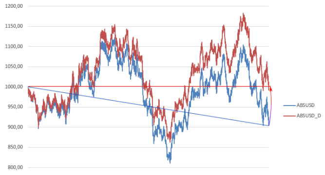
In the simple algorithm above, one clause requires an explanation: “preliminary processing of price data”. Let me explain with an example of the price chart for the ABS / USD asset (price distribution is lognormal), which we obtained earlier:
The final price of the ABS / USD asset is lower than the original price. The downtrend of our asset is not a pattern, but the influence of a non-deterministic factor - let me remind you that we used a random number generator.
At the same time, it is known a priori about the ABS / USD asset that its price, in general, drifts equally up or down. That is, in the model, the mathematical expectation of the ABS / USD price deviation is 0.
In the statistical evaluation, the mathematical expectation — the average value of the price change — turned out to be negative.
Is it correct to use for the calculations data that already contain a priori “knowledge” about the negative profitability of an asset? The word "knowledge" is not without reason put in quotes: we know that the ABS / USD asset is equally likely to grow in price and become cheaper. This is the data model we used in the calculation.
On the other hand, statistics show us a negative expectation of daily price dynamics. And this “knowledge” obtained on, in fact, a random sample, we will lay in the model.
ABS / USD is a hypothetical asset. It is definitely possible to say that, for the construction of the table - the distribution function, which will later be used to generate price forecasts, the current trend is a statistical error that needs to be eliminated.
But what if we analyze a real market asset? Not ABS / USD, but, for example, EUR / USD? How to deal with the trend that took place in reality?
My opinion: trend should be removed from price history. The opposite is true if we have "reliable" evidence that the price of an asset will continue to decline in the future. Yes, there are such currencies, goods and other objects of trade, on the dynamics of pricing which economic analysis gives a certain forecast. What can not be said, for example, about the majority of cryptocurrencies.
Where there are enough reasoned statements both in favor of the uptrend and in favor of the downtrend, the historical prices should be “aligned”:
In the figure, the original blue curve was adjusted: a value equal to i * d was subtracted from each i-th price value, where d is equal to the difference between the first and last prices divided by the number of time periods (the number of prices minus 1).
In an application program designed to estimate the value of the premium on an option contract, it is probably worthwhile to provide two calculation options: with the removal of the trend and with the data taken and used as is.
Certainly, where we do not have full confidence in the price dynamics for the forecast period, the trend should be eliminated. And if there is confidence - is it worth spending time studying derivatives, when you can just enter the market with all the available funds and, with a tangible profit, monetize your forecasts?
Another note: the trend does not necessarily eliminate directly from the prices. For example, bitcoin with its growth of more than one hundred percent in one year only after the removal of the trend component from prices will generally go into the negative half-plane along the price axis. The negative price is definitely not suitable for further calculations. The alternative I use is to remove the trend from a range of price changes - ln( fracxixi−1) where xiandxi−1xi - current and previous price values.
Construction and use of the inverse cumulative distribution function
In the program that I bring in the depository of the github code by reference , perhaps the most “intelligent” part is the construction of the inverse cumulative (integral) distribution function and using it to generate a random price increment. The whole process is divided into several steps.
In the first step I get from the prices x1,x2,...,xN increments d1,d2,...,dN−1:di=ln( fracxixi−1)
Further, if the option to eliminate the trend is selected, I get a new series of price increments, subtracting from each value di equal to fracdN−1−d1N−2 .
I sort the price increment values in ascending order.
The process of constructing the inverse distribution function is implemented in one cycle. Imagine that the price changes ( xi+1=xi∗edi a) on discrete values di . What is the probability that the price will change in ed1 or less times where d1 - the smallest of the price increment values in our sample? Obviously, this probability will be frac1N−1 . What is the probability that the price will change in ed2 or less times? Obviously, this probability is equal to the sum of the probabilities of two unrelated outcomes: price changes in ed1 times either in ed2 times or frac1+1N−1 .
Ie, having a sorted row d1,d2,...,dN−1 , it is enough for us to build from it a series of tuples
[d1, frac1N−1],[d2, frac2N−1],...[dN−1, fracN−1N−1]
.
So, the inverse function is constructed. How do we get the “random” value of the price change using a table and a generator of uniformly distributed random numbers?
About the same as we did in Excel.
For example, my table contains 500 records of the form:
| Probability P | Delta, D |
| 0.002 | -0.0172 |
| 0.004 | -0.0699 |
| ... | ... |
In the table constructed by the program, the 1st entry corresponds to the probability equal to 1/500, the second to 2/500, and so on.
I get a random fractional number in the range from 0 to 1. For example, 0.269.
I multiply a random number by the number of records in the table (500): 0.269 * 500 = 134.5.
The delta value I need will be “in the middle” between the 134th and 135th rows of the table:
D134+(D135−D134)∗(134.5−134.0)
As soon as we interpolate the value of the price increment, we calculate the new value of the price using the formula
pi+1=pi∗eD
Simulation results
Now my task is to verify the option premium calculation algorithm using the algorithm described above. Verify by the example of a calculation performed for the assets ABSUSD (lognormal) and WRDUSD (thick-tailed). Let me remind you: ABSUSD is characterized by price increments having a lognormal distribution. The very distribution that suggests the model B- . Asset WRDUSD demonstrates price movements closer to the real market.
In the program, I specified exactly the same parameters as for calculations in Excel. Instead of calculating the premium using a standard deviation formula, I passed the price time series of our assets to the program. The result shows the table:
| - | ABS / USD | WRD / USD |
| price distribution law | lognormal distribution | “Real” distribution |
| premium formula b-sh | 10.80 | 10.80 |
| premium derived from modeling price movements | 10.70 | 11.20 |
The calculation for the ABS / USD asset gives almost the same result as the formula B-Sh. But for the WRD / USD asset, the “simulated” premium is already noticeably different from the result of the analytical calculation.
There are two possible reasons for this: the very nature of the WRD / USD price range and / or sampling error .
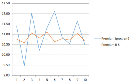
We have to be sure that the difference in the results of modeling and analytical calculation is due precisely to the nature of our virtual asset. To this end, I will spend 10 iterations of calculating the premium, generating 10 WRD / USD price series. For each such sample, I will calculate the standard deviation, substitute it in the formula B- and get the result of the analytical calculation:
It can be said that the sampling error more influenced the result of the program calculation than on the result of calculations using the formula -. In the course of 10 experiments, the average values of the premium size were obtained:
- program result: 11.0,
- according to the formula -: 10.83.
The differences in the result are minor. From which we can conclude: so far, the significant influence of the law of price distribution on the estimated value of the “fair” premium on the option contract was not found .
Calculation of premium on market contracts
So far, we have analyzed “virtual” assets, the dynamics of which obey the laws, which we formulated as well. The purpose of these surveys is to evaluate real assets. Option contracts for cryptocurrencies, the value of which is expressed in fiat currencies or other cryptocurrencies.
As before, let's take a vanilla 30-day option BTCUSD - Bitcoin exchange rate to the US dollar. Let's spend 4 iterations of calculation. For the first iteration, we take the entire BTCUSD quoting history from 2011 to 2017 as input. We calculate the premium, eliminating the trend from the original data. The current price is $ 10,709 for 1 bitcoin.
The award received analytically (B-), has made $ 1234 .
By modeling the price series in the program, we get a premium value of $ 1938 .
The discrepancy between the analytical result and the software in the case of BTCUSD is significant this time.
As the source data, we took the entire history of bitcoin quoting. In general, when calculating the premium on an option, it is customary to take not all the available data, but a relatively “fresh” price history. The same bitcoin went through a series of ups and downs in prices characteristic of a developing, “immature” market.
Obviously, it would be strange to build an estimate of the value of the option of today's popular and liquid asset, starting from the history of 7 years ago, when Bitcoin was a wonder, and its capitalization was insignificant.
Bitcoin sample of 2011 and the current bitcoin, from the point of view of the financial world - two different assets. Therefore, I will repeat the calculations, limiting myself to the period of 2014-2017, then the period of 2016-2017:
| - | HV ,% | Award ( program ) | Prize ( BS ) |
| 2011-2017 | 101.15 | 1938.34 | 1234.67 |
| 2014-2017 | 66.26 | 1127.22 | 810.40 |
| 2016-2017 | 62.96 | 1407.93 | 770.15 |
What can be attributed to such a significant discrepancy of the premium, calculated in two ways? Sampling error or poor applicability of the formula B-III for a volatile, “unpredictable” cryptoactive?
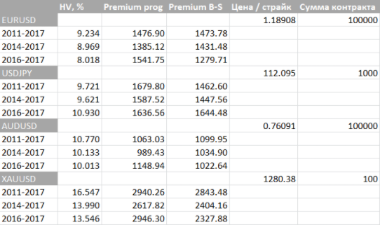
For comparison, I will give the data on the calculation of the option premium on popular currency pairs / gold:
For the “mature” markets, as can be seen from the table, the discrepancies in the simulation results with the formula B – SH are not as significant as for BTCUSD (Bitcoin).
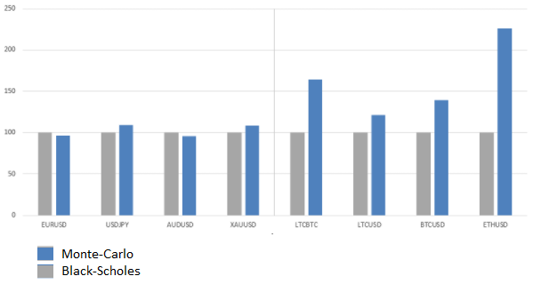
The following diagram shows how the calculated premium values (program / formula B-Sh) for fiat currencies , gold, and cryptocurrencies differ:
Recommendations for the practical evaluation of an option contract premium
When calculating the option premium of an asset as unpredictable and dynamic as a cryptocurrency, it is worth considering a number of factors.
First, we can assume a strong influence of the sampling error on the calculation of the premium. This assumption clearly confirms the experiment with ten samples of an artificial time series WRDUSD.
Secondly, the assessment of the “fair” premium, obtained by software modeling at different intervals of the asset's price history, may differ significantly from the estimate calculated by the formula B- from historical volatility. Personally, I prefer a more conservative , albeit, probably, too high, estimate, obtained by modeling the price series.
Thirdly, the same asset in different periods may be characterized by different dynamics. Generally speaking, there is a more general model of price dynamics with respect to the model BS-H, the model of Heston, which implies the “drifting” volatility of an asset. In the case of cryptocurrency assets, the Heston model is likely to be redundantly complex and not quite adequate (under certain conditions). Instead of the assumption of a stochastic one that tends to return to the average value of volatility, it is more logical to assume that cryptocurrency price volatility changes with time, “evolves”, back correlating with the growth of market capitalization.
Finally, in my assessment, I assume my complete ignorance about the emerging price trend . The premium estimate for the “vanilla” CALL option, obtained without eliminating the trend, will exceed the premium estimate of the PUT option by 40% - 70%. Even if I decide to leave the trend in historical data, the cryptoactive growth scenario is just one of the possible scenarios. Choosing from two alternatives, for example, I can dwell on the “weighted” value of the premium:
C=CT∗PT+CD∗(1−PT)
,
Where
- C - premium (it does not matter if the call or put option is available),
- CT - premium calculated by the data in which the trend is saved,
- CD - premium calculated by the data after the removal of the trend,
- PT - My estimate of the probability of maintaining the current trend.
And the last one in the list, but the first one in importance is the principle by which I am guided: speaking about the “fair” premium on the option, I take the word “fair” in quotes. Speaking about the probability calculated by the history of observations, I am not talking about probability as such, but about its assessment . The rigor of formulations helps me to maintain at least some critical attitude toward my own (and even to others') even more so) predictions and assumptions.
Source: https://habr.com/ru/post/345362/
All Articles