Creating a Christmas animation with Wolfram Language
Translation of the blog O Tannenbaum Michael Trotta, director of Wolfram | Alpha.
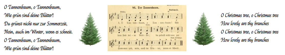
This laptop describes how to create an animation of a decorated Christmas tree that moves its branches in sync with the voices of the music of the German song O Tannenbaum of the 16th century (English version - O Christmas Tree ). One selected branch of the tree will act as a conductor, and the candle will be a baton. This makes the animation interesting in all the verses. We will also add some snow and some funny tree movements in the second half of the song. To see the final design, watch this YouTube video :
')

I implement the animation using the following steps:
- Build a Christmas tree with curved branches, where the branches can be moved smoothly up, down, left and right.
- Add decorations (colored balls, five-pointed stars) and candles of different colors to the branches. Allow the jewelry to move relative to the ends of the branches.
- Convert 4 voices of music to 2D motion based on sound frequencies. Simulate the conductor's movements synchronized with the music.
- Simulate the movement of jewelry in the form of a spherical pendulum. Accounting friction patterns using dissipative function Rayleigh.
- Add snow for white christmas.
- Create a branch animation in relation to music.
Special thanks to my colleague Andrew Steyhacher for selecting and analyzing music in order to obtain data for the movement of the tree (below the section “From music to movements”). And thanks to Amy Young for turning animated frames and music into one video clip.
Creating a Christmas tree
Tree options
The size of the tree, the overall shape of the tree and the number of branches. The names of the variables make their meaning obvious.
(* radial branch count *) radialBranchCount = 3; (* vertical branch count *) verticalBranchCount = 5; (* tree height *) treeHeight = 12; (* tree width *) treeWidth = 6; (* plot points for the B-spline surfaces forming the branches *) {μ, ν} = {6, 8}; The colors of the trunk and branches.
stemColor = Directive[Darker[Brown], Lighting -> "Neutral", Specularity[Brown, 20]]; branchTopColor = RGBColor[0., 0.6, 0.6]; branchBottomColor = RGBColor[0., 0.4, 0.4]; branchSideColor = RGBColor[0.4, 0.8, 0.]; Building a moving tree branch
Each branch has a cross section of a rectangle with varying dimension (depending on the distance from the stem). The tip of the branch should point slightly upwards in order to have the familiar look of the Christmas tree. At its widest size, the branch lies close to the cone (trunk). The variable τ defines the up-down and variable σ left-right position of the branch tip. I build a branch from the four surfaces of the B-spline (top, bottom, left, right) to have a smooth appearance with a small number of points defining the surface.
branchTopBottom[ tp_, {hb_, ht_}, {φ1_, φ2_}, {rb_, rt_}, R_, {σ_, τ_}] := Module[{A = -0.6, β = 1/2, φm, Pm, dirR, dirφ, r, P1, P, \[ScriptN], \[ScriptP], x, y, ω, ℛ, ξ, \[ScriptH]s, \[ScriptH]}, φm = Mean[{φ1, φ2}]; Pm = R {Cos[φm], Sin[φm]}; dirR = 1. {Cos[φm], Sin[φm]}; dirφ = Reverse[dirR] {-1, 1}; r = If[tp == "top", rt, rb]; (* move cross section radially away from the stem and contract it *) Table[P1 = {r Cos[φ], r Sin[φ]}; Table[P = P1 + s/ν (Pm - P1); \[ScriptN] = dirφ.P; \[ScriptP] = dirR.P; {x, y} = \[ScriptN] Cos[ s/ν Pi/2]^2 dirφ + \[ScriptP] dirR; ω = σ* 1. s/ν Abs[φ2 - φ1]/ radialBranchCount; ℛ = {{Cos[ω], Sin[ω]}, {-Sin[ω], Cos[ω]}}; {x, y} = ℛ.{x, y}; ξ = R s/ν; \[ScriptH]s = {ht, hb} + {ξ (AR (R - ξ) - (hb - ht) (β - 1) ξ), (ht - hb) ξ^2 β}/R^2; \[ScriptH] = If[tp == "top", \[ScriptH]s[[1]], \[ScriptH]s[[2]]] ; {x, y, \[ScriptH] + τ s/ν (ht - hb)}, {s, 0, ν}], {φ, φ1, φ2, (φ2 - φ1)/μ}] // N ] The radius at height h is only a linear interpolation of the maximum trunk radius and radius 0 in the upper part.
stemRadius[h_, H_] := (H - h)/H The sides of the branch are only connecting elements between the upper and lower surfaces.
branchOnStem[{{hb_, ht_}, {φ1_, φ2_}, R_}, {τ_, σ_}] := Module[{tBranch, bBranch, sideBranches}, {bBranch, tBranch} = Table[branchTopBottom[p, {hb, ht}, {φ1, φ2}, stemRadius[{hb, ht}, treeHeight], R, {τ, σ}], {p, {"top", "bottom"}}]; sideBranches = Table[BSplineSurface[{tBranch[[j]], bBranch[[j]]}], {j, {1, -1}}]; {branchTopColor, BSplineSurface[tBranch], branchBottomColor, BSplineSurface[bBranch], branchSideColor, sideBranches} ] For later use, let's define a function only for the position of the end of the branch.
branchOnStemEndPoint[ {{hb_, ht_}, {φ1_, φ2_}, R_}, {σ_, τ_}] := Module[{A = -0.6, β = 1/2, Pm, dirR, dirφ, P, \[ScriptN], \[ScriptP], x, y, ω, ξ, \[ScriptH]s, \[ScriptH], φ = φ1, φm = Mean[{φ1, φ2}]}, Pm = R {Cos[φm], Sin[φm]}; dirR = {Cos[φm], Sin[φm]}; {x, y} = dirR.Pm dirR; ω = 1. σ Abs[φ2 - φ1]/radialBranchCount; {x, y} = {{Cos[ω], Sin[ω]}, {-Sin[ω], Cos[ω]}}.{x, y}; \[ScriptH]s = {ht, hb} + (ht - hb) {β - 1., 1}; {x, y, \[ScriptH]s[[1]] + τ (ht - hb)} ] An interactive demonstration that allows a branch and its end to move as a function of {σ, τ}.
Manipulate[ Graphics3D[{branchOnStem[{{0, 1}, {Pi/2 - 1/2, Pi/2 + 1/2}, 1 + ρ}, στ], Red, Sphere[branchOnStemEndPoint[{{0, 1}, {Pi/2 - 1/2, Pi/2 + 1/2}, 1 + ρ}, στ], 0.05]}, PlotRange -> {{-2, 2}, {0, 4}, {-1, 2}}, ViewPoint -> {3.17, 0.85, 0.79}], {{ρ, 1.6, "branch length"}, 0, 2, ImageSize -> Small}, {{στ, {0, 0}, "branch\nleft/right\nup/down"}, {-1, -1}, {1, 1}}, ControlPlacement -> Left, SaveDefinitions -> True] 
Adding branches to the trunk
The trunk is just a cone, the top of which is the top of the tree.
stem = Cone[{{0, 0, 0}, {0, 0, treeHeight}}, 1]; The size of the branches decreases with height, becoming geometrically smaller. The total number of all levels of branches is equal to the height of the tree minus part of the step below.
heightList1 = Module[{α = 0.8, hs, sol}, hs = Prepend[Table[C α^k, {k, 0, verticalBranchCount - 1}], 0]; sol = Solve[Total[hs] == 10, C, Reals]; Accumulate[hs /. sol[[1]]]] {0, 2.97477, 5.35459, 7.25845, 8.78153, 10.}
treeWidthOfHeight[h_] := treeWidth (treeHeight - h)/treeHeight The branches are tight to the trunk, without gaps between them.
Graphics3D[{{stemColor, stem}, {Darker[Green], Table[Table[ branchOnStem[{2 + heightList1[[{j, j + 1}]], {k , k + 1} 2 Pi/ radialBranchCount , treeWidthOfHeight[Mean[heightList1[[{j, j + 1}]]]]}, {0, 0}], {k, 0, 1}] , {j, 1, verticalBranchCount}]}}, ViewPoint -> {2.48, -2.28, 0.28}] 
Graphics3D[{{stemColor, stem}, {Darker[Green], Table[Table[ branchOnStem[{2 + heightList1[[{j, j + 1}]], {k , k + 1} 2 Pi/ radialBranchCount , treeWidthOfHeight[Mean[heightList1[[{j, j + 1}]]]]}, {0, 0}], {k, 0, radialBranchCount - 1}] , {j, 1, verticalBranchCount}]}}, ViewPoint -> {2.48, -2.28, 0.28}] 
You can move branches to get a more realistic tree shape. This is the tree that I will use in the future. Changing tree settings and using another tree is quite simple.
heightList2 = {2/3, 1/3}.# & /@ Partition[heightList1, 2, 1]; Graphics3D[{{Darker[Brown], stem}, {EdgeForm[], Table[ Table[branchOnStem[ {2 + heightList1[[{j, j + 1}]], {k , k + 1} 2 Pi/ radialBranchCount , treeWidthOfHeight[Mean[heightList1[[{j, j + 1}]]]]}, {0, 0}], {k, 0, radialBranchCount - 1}] , {j, 1, verticalBranchCount}], Table[Table[ branchOnStem[{2 + heightList2[[{j, j + 1}]], {k , k + 1} 2 Pi/ radialBranchCount + Pi/radialBranchCount, treeWidthOfHeight[Mean[heightList2[[{j, j + 1}]]]]}, {0, 0}], {k, 0, radialBranchCount - 1}] , {j, 1, verticalBranchCount - 1}]}}, ViewPoint -> {2.48, -2.28, 0.28}] 
One could easily make trees even denser with more branches.
Graphics3D[{{Darker[Brown], stem}, {EdgeForm[], Table[Table[branchOnStem[ {2 + heightList1[[{j, j + 1}]], {k , k + 1} 2 Pi/(2 radialBranchCount) , treeWidthOfHeight[Mean[heightList1[[{j, j + 1}]]]]}, {0, 0}], {k, 0, (2 radialBranchCount) - 1}] , {j, 1, verticalBranchCount}], Table[Table[branchOnStem[{2 + heightList2[[{j, j + 1}]], {k , k + 1} 2 Pi/(2 radialBranchCount) + Pi/(2 radialBranchCount), treeWidthOfHeight[Mean[heightList2[[{j, j + 1}]]]]}, {0, 0}], {k, 0, 2 radialBranchCount - 1}] , {j, 1, verticalBranchCount - 1}]}}, ViewPoint -> {2.48, -2.28, 0.28}] 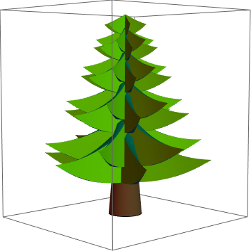
Tree decoration
Now let's build some decorations to build a beautifully decorated Christmas tree. I will add shiny balls, five-pointed stars and candles. I recommend the original Thuringian Laus balls for your Christmas tree. (You can find them here )
Jewelry, Candles and Top
Colored balls
Each tree should have some shiny glass spheres, toys.
coloredBall[p_, size_, color_, {ϕ_, θ_}] := Module[{\[ScriptD] = {Cos[ϕ] Sin[θ], Sin[ϕ] Sin[θ], -Cos[θ]}}, {EdgeForm[], GrayLevel[0.4], Specularity[Yellow, 20], Cylinder[{p, p + 1.5 size \[ScriptD]}, 0.02 size ], color, Specularity[Yellow, 10], Sphere[p + (1.5 size + 0.6 size) \[ScriptD] , 0.6 size] }] Graphics3D[{coloredBall[{1, 2, 3}, 1, Red, {0, 0}], coloredBall[{3, 2, 3}, 1, Darker[Blue], {1, 0.2}]}, Axes -> True] 
branchOnStemWithBall[{{hb_, ht_}, {φ1_, φ2_}, R_}, {σ_, τ_}, color_, {ϕ_, θ_}] := {branchOnStem[{{hb, ht}, {φ1, φ2}, R}, {σ, τ}] , coloredBall[ branchOnStemEndPoint[{{hb, ht}, {φ1, φ2}, R}, {σ, τ}], 0.45 (ht - hb)/2, color, {ϕ, θ}]} Here is a branch with a toy. The variables {σ, τ} allow changing the position of the ball relative to the tip of the branch.
Manipulate[ Graphics3D[{branchOnStemWithBall[{{0, 1}, {Pi/2 - 1/2, Pi/2 + 1/2}, 1 + ρ}, στ, Red, ϕθ]}, PlotRange -> {{-2, 2}, {0, 4}, {-2, 2}}, ViewPoint -> {3.17, 0.85, 0.79}], {{ρ, 1.6, "branch length"}, 0, 2, ImageSize -> Small}, {{στ, {0.6, 0.26}, "branch\nleft/right\nup/down"}, {-1, -1}, {1, 1}}, {{ϕθ, {2.57, 1.88}, "ball angles"}, {0, -Pi}, {Pi, Pi}}, ControlPlacement -> Left, SaveDefinitions -> True] 
Here is a tree with balls weighing mostly straight down. I will use random colors for the balls.
Graphics3D[{{Darker[Brown], stem}, {Table[ Table[branchOnStemWithBall[{2 + heightList1[[{j, j + 1}]], {k , k + 1} 2 Pi/ radialBranchCount , treeWidthOfHeight[Mean[heightList1[[{j, j + 1}]]]]}, {0, 0}, RandomColor[], {0, 0}], {k, 0, radialBranchCount - 1}] , {j, 1, verticalBranchCount}] }}, ViewPoint -> {2.48, -2.28, 0.28}, Axes -> True] 
Tree with balls in random directions. If later the branches are moved, then we calculate the natural movements (which means solving the corresponding equations of motion) of the balls.
Graphics3D[{{Darker[Brown], stem}, {Table[ Table[branchOnStemWithBall[{2 + heightList1[[{j, j + 1}]], {k , k + 1} 2 Pi/ radialBranchCount , treeWidthOfHeight[Mean[heightList1[[{j, j + 1}]]]]}, {0, 0}, RandomColor[], {RandomReal[{-Pi, Pi}], RandomReal[{0, Pi}]}], {k, 0, radialBranchCount - 1}] , {j, 1, verticalBranchCount}]}}, ViewPoint -> {2.48, -2.28, 0.28}, Axes -> True] 
Five-pointed stars
Now we build several five-pointed stars. Since this ornament does not have rotational symmetry, I will allow an orientation angle relative to the thread on which it hangs.
coloredFiveStar[p_, size_, dir_, color_, α_, {ϕ_, θ_}] := Module[{\[ScriptD] = {Cos[ϕ] Sin[θ], Sin[ϕ] Sin[θ], -Cos[θ]}, points, P1, P2, d1, d2, d3, dP, dP2}, d2 = Normalize[dir - dir.\[ScriptD] \[ScriptD]]; d3 = Cross[\[ScriptD], d2]; {EdgeForm[], GrayLevel[0.4], Specularity[Pink, 20], Cylinder[{p, p + (1.5 size + 0.6 size) \[ScriptD]}, 0.02 size ], color, Specularity[Hue[.125], 5], dP = Sin[α] d2 + Cos[α] d3; dP2 = Cross[\[ScriptD], dP]; points = Table[p + (1.5 size + 0.6 size) \[ScriptD] + size If[EvenQ[j], 1, 1/2] * (Cos[j 2 Pi/10 ] \[ScriptD] + Sin[j 2 Pi/10] dP), {j, 0, 10}]; P1 = p + (1.5 size + 0.6 size) \[ScriptD] + size/3 dP2; P2 = p + (1.5 size + 0.6 size) \[ScriptD] - size/3 dP2; {P1, P2} = (p + (1.5 size + 0.6 size) \[ScriptD] + # size/ 3 dP2) & /@ {+1, -1}; Polygon[ Join @@ (Function[a, Append[#, a] & /@ Partition[points, 2, 1]] /@ {P1, P2})] }] Graphics3D[{coloredFiveStar[{1, 2, 3}, 0.2, {0, -1, 0}, Darker[Red], 0, {0, 0}], coloredFiveStar[{1.5, 2, 3}, 0.2, {0, -1, 0}, Darker[Purple], Pi/3, {1, 0.4}]}] 
branchOnStemWithFiveStar[{{hb_, ht_}, {φ1_, φ2_}, R_}, {σ_, τ_}, color_, α_, {ϕ_, θ_}] := Module[{dir = Append[Normalize[ Mean[{{Cos[φ1], Sin[φ1]}, {Cos[φ2], Sin[φ2]}}]], 0]}, {branchOnStem[{{hb, ht}, {φ1, φ2}, R}, {σ, τ}] , coloredFiveStar[ branchOnStemEndPoint[{{hb, ht}, {φ1, φ2}, R}, {σ, τ}], 0.4 (ht - hb)/2, dir, color, α, {ϕ, θ}]} ] The Christmas tree is decorated with five-pointed stars.
Graphics3D[{{Darker[Brown], stem}, {Table[ Table[branchOnStemWithFiveStar[{2 + heightList1[[{j, j + 1}]], {k , k + 1} 2 Pi/ radialBranchCount , treeWidthOfHeight[Mean[heightList1[[{j, j + 1}]]]]}, {0, 0}, RandomColor[], RandomReal[{-Pi, Pi}], {RandomReal[{-Pi, Pi}], RandomReal[0.1 {-1, 1}]}], {k, 0, radialBranchCount - 1}] , {j, 1, verticalBranchCount}] }}, ViewPoint -> {2.48, -2.28, 0.28}, Axes -> True] 
Candles
We will construct them starting from the leg, which is attached to the ends of the branches, with a wax-like body, blackened wick and fire. To ease the animation and avoid the fire, I will use electric candles so that the flame does not change when the branches move.
flamePoints = Table[{0.2 Sin[Pi z]^2 Cos[φ], 0.2 Sin[Pi z]^2 Sin[φ], z}, {z, 0, 1, 1/1/12}, {φ, Pi/2, 5/2 Pi, 2 Pi/24}] litCandle[p_, size_, color_] := {EdgeForm[], color, Cylinder[{p + {0, 0, size 0.001}, p + {0, 0, size 0.5}}, size 0.04], GrayLevel[0.1], Specularity[Orange, 20], Cylinder[{p, p + {0, 0, size 0.05}}, size 0.06], Black, Glow[Black], Cylinder[{ p + {0, 0, size 0.5}, p + {0, 0, size 0.5 + 0.05 size}}, size 0.008], Glow[Orange], Specularity[Hue[.125], 5], BSplineSurface[ Map[(p + {0, 0, size 0.5} + 0.3 size #) &, flamePoints, {2}], SplineClosed -> {True, False}] } White and red candles.
Graphics3D[{litCandle[{0, 0, 0}, 1, Directive[White, Glow[GrayLevel[0.3]], Specularity[Yellow, 20]]], litCandle[{0.5, 0, 0}, 1, Directive[Red, Glow[GrayLevel[0.1]], Specularity[Yellow, 20]]]}] 
Later I will use an elongated branch with a candle so that it will be the conductor, so I will allow the candles to lean from the branch.
branchOnStemWithCandle[{{hb_, ht_}, {φ1_, φ2_}, R_}, {σ_, τ_}, color_, α_] := {branchOnStem[{{hb, ht}, {φ1, φ2}, R}, {σ, τ}] , If[α == 0, litCandle[ branchOnStemEndPoint[{{hb, ht}, {φ1, φ2}, 0.98 R}, {σ, τ}], 0.66 (ht - hb) , color], Module[{P = branchOnStemEndPoint[{{hb, ht}, {φ1, φ2}, 0.98 R}, {σ, τ}], dir}, dir = Append[Reverse[Take[P, 2]] {-1, 1}, 0]; Rotate[ litCandle[ branchOnStemEndPoint[{{hb, ht}, {φ1, φ2}, 0.98 R}, {σ, τ}], 0.66 (ht - hb) , color], α, dir, P]]]} Manipulate[ Graphics3D[{branchOnStemWithCandle[{{0, 1}, {Pi/2 - 1/2, Pi/2 + 1/2}, 1 + ρ}, στ, Red, α]}, PlotRange -> {{-2, 2}, {0, 4}, {-2, 2}}, ViewPoint -> {3.17, 0.85, 0.79}], {{ρ, 1.6, "branch length"}, 0, 2, ImageSize -> Small}, {{στ, {0, 0}, "branch\nleft/right\nup/down"}, {-1, -1}, {1, 1}}, {{α, Pi/4, "candle angle"}, -Pi, Pi}, ControlPlacement -> Left, SaveDefinitions -> True] And here is a spruce with a candle on each branch.
Graphics3D[{{Darker[Brown], stem}, {Table[ Table[branchOnStemWithCandle[{2 + heightList1[[{j, j + 1}]], {k , k + 1} 2 Pi/ radialBranchCount , treeWidthOfHeight[Mean[heightList1[[{j, j + 1}]]]]}, {0, 0}, White, 0], {k, 0, radialBranchCount - 1}] , {j, 1, verticalBranchCount}] }}, ViewPoint -> {2.48, -2.28, 0.28}, Axes -> True] 
The top of the tree
For complete joy, I add a rotating spike on the top.
spikey = Cases[ N@Entity["Polyhedron", "RhombicHexecontahedron"][ "Image"], _GraphicsComplex, ∞][[1]]; top = {Gray, Specularity[Red, 25], Cone[{{0, 0, 0.9 treeHeight}, {0, 0, 1.08 treeHeight}}, treeWidth/240], Orange, EdgeForm[Darker[Orange]], Specularity[Hue[.125], 5], MapAt[((0.24 # + {0, 0, 1.08 treeHeight}) & /@ #) &, spikey, 1] } Graphics3D[{{Darker[Brown], stem}, {Table[ Table[branchOnStem[{2 + heightList1[[{j, j + 1}]], {k , k + 1} 2 Pi/ radialBranchCount , treeWidthOfHeight[Mean[heightList1[[{j, j + 1}]]]]}, {0, 0} ], {k, 0, radialBranchCount - 1}] , {j, 1, verticalBranchCount}], top}}, ViewPoint -> {2.48, -2.28, 0.28}, Axes -> True] 
Tree decoration
We will single out one branch as a conductor. We will randomly divide the remaining branches into four groups and decorate them with toys of two colors, five-pointed stars and candles.
Now let's add a decoration or a candle to each branch of the tree. I will use the above tree with 27 branches. I start branches in height on the stem and azimuth angle.
allBranches = Flatten[Riffle[ Table[Table[{2 + heightList1[[{j, j + 1}]], {k , k + 1} 2. Pi/ radialBranchCount , treeWidthOfHeight[Mean[heightList1[[{j, j + 1}]]]]}, {k, 0, radialBranchCount - 1}] , {j, 1, verticalBranchCount}], Table[Table[{2 + heightList2[[{j, j + 1}]], {k , k + 1} 2. Pi/ radialBranchCount + Pi/radialBranchCount, treeWidthOfHeight[Mean[heightList2[[{j, j + 1}]]]]}, {k, 0, radialBranchCount - 1}] , {j, 1, verticalBranchCount - 1}]], 1] Length[allBranches] 27
Let's color the branches in order, starting from the red below and to the purple on the top.
Graphics3D[{{Darker[Brown], stem}, MapIndexed[(branchOnStem[#1, {0, 0}] /. _RGBColor :> Hue[#2[[1]]/36]) &, allBranches], top}, ViewPoint -> {2, 1, -0.2}] 
We divide all branches into 4 groups for voices and one for the role of conductor.
conductorBranch = 7; SeedRandom[12]; voiceBranches = (Last /@ #) & /@ GroupBy[{RandomChoice[{1, 2, 3, 4}], #} & /@ Delete[Range[27], {conductorBranch}], First] <| 1 -> {1, 4, 5, 6, 12, 18, 20}, 3 -> {2, 8, 10, 11, 14, 22, 23, 25}, 2 -> {3, 13, 15, 16, 21, 26}, 4 -> {9, 17, 19, 24, 27} |>
voiceBranches = <|1 -> {2, 9, 14, 17, 19, 24, 27}, 2 -> {3, 13, 15, 16, 21, 26}, 3 -> {1, 4, 5, 12, 18, 20}, 4 -> {6, 8, 10, 11, 22, 23, 25}|> <| 1 -> {2, 9, 14, 17, 19, 24, 27}, 2 -> {3, 13, 15, 16, 21, 26}, 3 -> {1, 4, 5, 12, 18, 20}, 4 -> {6, 8, 10, 11, 22, 23, 25} |>
Here is an illustration of branches, painted according to what voice they represent.
Graphics3D[{{Darker[Brown], stem}, branchOnStem[#1, {0, 0}] & /@ allBranches[[voiceBranches[[1]]]] /. _RGBColor :> Yellow, branchOnStem[#1, {0, 0}] & /@ allBranches[[voiceBranches[[2]]]] /. _RGBColor :> White, branchOnStem[#1, {0, 0}] & /@ allBranches[[voiceBranches[[3]]]] /. _RGBColor :> LightBlue, branchOnStem[#1, {0, 0}] & /@ allBranches[[voiceBranches[[4]]]] /. _RGBColor :> Pink, branchOnStem[ allBranches[[conductorBranch]] {1, 1, 1.5}, {0, 0}] /. _RGBColor :> Red, top}, ViewPoint -> {2, 1, -0.2}] 
A completed tree with the location of the end of the branches as parameters. Also let the decorations on the tips of the branches sit tilted and be colorful.
christmasTree[{{σ1_, τ1_}, {σ2_, τ2_}, {σ3_, τ3_}, {σ4_, τ4_}, {σc_, τc_}}, {{ϕ1_, θ1_}, {ϕ2_, θ2_}, {ϕ3_, θ3_}}, {colBall1_, colBall2_, col5Star_}, conductorEnhancementFactor : fc_, conductorCandleAngle : ωc_, topRotationAngle : ω_] := {{Darker[Brown], stem}, branchOnStemWithBall[#, {σ1, τ1}, colBall1, {ϕ1, θ1}] & /@ allBranches[[voiceBranches[[1]]]], branchOnStemWithBall[#, {σ2, τ2}, colBall2, {ϕ2, θ2}] & /@ allBranches[[voiceBranches[[2]]]], branchOnStemWithFiveStar[#, {σ3, τ3}, col5Star, Pi/4, {ϕ3, θ3}] & /@ allBranches[[voiceBranches[[3]]]], branchOnStemWithCandle[#, {σ4, τ4}, Directive[White, Glow[GrayLevel[0.3]], Specularity[Yellow, 20]], 0] & /@ allBranches[[voiceBranches[[4]]]], branchOnStemWithCandle[ allBranches[[conductorBranch]] {1, 1, 1 + fc}, {σc, τc}, Directive[Red, Glow[GrayLevel[0.1]], Specularity[Yellow, 20]], ωc], Rotate[top, ω, {0, 0, 1}] }; The initial position of all branches and the elongated branch of the conductor, where its candle is tilted.
Graphics3D[christmasTree[{{0, 0}, {0, 0}, {0, 0}, {0, 0}, {0, 0}}, {{0, 0}, {0,0}, {0, 0}}, {Red, Darker[Yellow], Pink}, 0.8, Pi/4, 0], ImageSize -> 600, ViewPoint -> {3.06, 1.28, 0.27}, PlotRange -> {{-7, 7}, {-7, 7}, {0, 15}}] 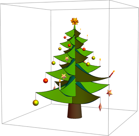
Three ate with all the parameters selected randomly.
SeedRandom[1] Table[Graphics3D[christmasTree[RandomReal[1.5 {-1, 1}, {5, 2}], Table[{RandomReal[{-Pi, Pi}], RandomReal[{0, Pi}]}, 3], RandomColor[3], RandomReal[], RandomReal[Pi/2], 0], ImageSize -> 200, ViewPoint -> {3.06, 1.28, 0.27}, PlotRange -> {{-7, 7}, {-7, 7}, {-2, 15}}], {3}] // Row 
The following interactive demonstrations allow you to move branches, move decorations around the ends of branches, and color decorations as you like.
Manipulate[ Graphics3D[ christmasTree[{στ1, στ2, στ3, στ4, στc}, {ϕθ1, ϕθ2, ϕθ3}, {col1, col2, col3}, l, ωc, ω], ImageSize -> 400, ViewPoint -> {2.61, 1.99, 0.80}, PlotRange -> {{-7, 7}, {-7, 7}, {-2, 15}}], "conductor", {{l, 0.6, "branch length"}, 0, 1, ImageSize -> Small}, {{ωc, Pi/4, "candle angle"}, 0, Pi, ImageSize -> Small}, {{στc, {0, 0}, "movement"}, {-1, -1}, {1, 1}, ImageSize -> Small}, Delimiter, "voice 1 (balls)", Grid[{{"movement", "ornament"}, {Control[{{στ1, {0, 0}, ""}, {-1, -1}, {1, 1}, ImageSize -> Small}], Control[{{ϕθ1, {0, 0}, ""}, {-Pi, 0}, {Pi, Pi}, ImageSize -> Small}]}}], {{col1, Red, ""}, Red, ImageSize -> Tiny}, Delimiter, "voice 2 (balls)", Grid[{{"movement", "ornament"}, {Control[{{στ2, {0, 0}, ""}, {-1, -1}, {1, 1}, ImageSize -> Small}], Control[{{ϕθ2, {0, 0}, ""}, {-Pi, 0}, {Pi, Pi}, ImageSize -> Small}]}}], {{col2, Darker[Yellow], ""}, Red, ImageSize -> Tiny}, Delimiter, "voice 3 (5-star)", Grid[{{"movement", "ornament"}, {Control[{{στ3, {0, 0}, ""}, {-1, -1}, {1, 1}, ImageSize -> Small}], Control[{{ϕθ3, {0, 0}, ""}, {-Pi, 0}, {Pi, Pi}, ImageSize -> Small}]}}], {{col3, Pink, ""}, Red, ImageSize -> Tiny}, Delimiter, "voice 4 (white candles)", Control[{{στ4, {0, 0}, "movement"}, {-1, -1}, {1, 1}, ImageSize -> Small}], Delimiter, Delimiter, {{ω, 0, "top rotation"}, 0, 1, ImageSize -> Small}, ControlPlacement -> Left, SaveDefinitions -> True] 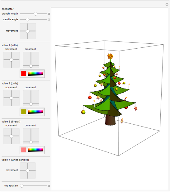
From music to movement
So, now that I’ve finished making a parameterized Christmas tree with moving branches and decorations, I have to deal with the ratio of music to branch movements (and, in turn, decorations).
Get 4 voices as sound
Use the MIDI file of the song.

{ohTannenBaum // Head, ohTannenBaum // ByteCount} {Sound, 287816}
Remove 4 voices.
voices = AssociationThread[{"Soprano", "Alto", "Tenor", "Bass"}, ImportString[ ExportString[ohTannenBaum, "MIDI"], {"MIDI", "SoundNotes"}]]; Sound[Take[#, 10]] & /@ voices 
Voice to frequency
frequencyRules = <|"A1" -> 55., "A2" -> 110., "A3" -> 220., "A4" -> 440., "B1" -> 61.74, "B2" -> 123.5, "B3" -> 246.9, "B4" -> 493.9, "C2" -> 65.41, "C3" -> 130.8, "C4" -> 261.6, "C5" -> 523.3, "D2" -> 73.42, "D#4" -> 311.13, "D4" -> 293.7, "D5" -> 587.3, "E2" -> 82.41, "E4" -> 329.6, "E5" -> 659.3, "F#2" -> 92.50, "F#4" -> 370.0, "G2" -> 98.00, "G#4" -> 415.3, "G4" -> 392.0|>; {minf, maxf} = MinMax[frequencyRules] {55., 659.3}
The timing of the first vote.
pw[t_] = Piecewise[{frequencyRules[#1], #2[[1]] <= t <= #2[[2]]} & @@@ voices[[1]]]; Plot[pw[t], {t, 0, 100}, PlotRange -> {200, All}, Filling -> Axis, PlotLabel -> "Soprano", Frame -> True, FrameLabel -> {"time in sec", "frequency in Hz"}, AxesOrigin -> {0, 200}] 
To represent the frequencies in the movements, I will smooth the curves.
spline = BSplineFunction[Table[{t, pw[t]}, {t, 0, 100, 0.5}], SplineDegree -> 2] 
ParametricPlot[spline[t], {t, 0, 100}, AspectRatio -> 0.5, PlotPoints -> 1000] 
tMax = 100; Do[ With[{j = j}, pwf[j][t_] = Piecewise[{frequencyRules[#1], #2[[1]] <= t <= #2[[2]]} & @@@ voices[[j]]]; splineFunction[j] = BSplineFunction[Table[{t, pwf[j][t]}, {t, 0, 100, 0.5}], SplineDegree -> 2]; voiceFunction[j][t_Real] := If[0 < t < tMax, splineFunction[j][t/tMax][[2]]/maxf, 0]], {j, 4}] Frequencies of four voices.
Plot[Evaluate[Reverse@Table[pwf[j][t], {j, 4}]], {t, 0, 100}, Frame -> True, FrameLabel -> {"time in sec", "frequency in Hz"}, AspectRatio -> 0.3] 
Smoothed scaled frequencies of four voices.
Plot[Evaluate[Table[voiceFunction[j][t], {j, 4}]], {t, 0, 100}, Frame -> True, FrameLabel -> {"time in sec", "scaled frequency"}, AspectRatio -> 0.3] 
Here is a graph of the (smoothed) first three voices in 3D.
ParametricPlot3D[{voiceFunction[1][t], voiceFunction[2][t], voiceFunction[3][t]}, {t, 0, 100}, AspectRatio -> Automatic, PlotPoints -> 1000, BoxRatios -> {1, 1, 1}] 
Show[% /. Line[pts_] :> Tube[pts, 0.002], Method -> {"TubePoints" -> 4}] 
Get a pattern of oscillation
Snap to specific phrases to create all the beatings of tact.
{firstBeat, secondBeat, lastBeat} = voices["Soprano"][[{1, 2, -1}, 2, 1]] {1.33522, 2.00568, 98.7727}
anchorDataOChristmasTree = SequenceCases[ voices["Soprano"], (* pattern for "O Christmas Tree, O Christmas Tree..." *) { SoundNote["D4", {pickupStart_, _}, "Trumpet", ___], SoundNote["G4", {beatOne_, _}, "Trumpet", ___], SoundNote["G4", {_, _}, "Trumpet", ___], SoundNote["G4", {beatTwo_, _}, "Trumpet", ___], SoundNote["A4", {beatThree_, _}, "Trumpet", ___], SoundNote["B4", {beatFour_, _}, "Trumpet", ___], SoundNote["B4", {_, _}, "Trumpet", ___], SoundNote["B4", {beatFive_, _}, "Trumpet", ___] } :> <| "PhraseName" -> "O Christmas Tree", "PickupBeat" -> pickupStart, "TargetMeasureBeats" -> {beatOne, beatTwo, beatThree}, "BeatLength" -> Mean@Differences[{pickupStart, beatOne, beatTwo, beatThree, beatFour, beatFive}] |> ]; anchorDataYourBoughsSoGreen = SequenceCases[ voices["Soprano"], (* "Your boughs so green in summertime..." *) { SoundNote["D5", {pickupBeatAnd_, _}, "Trumpet", ___], SoundNote["D5", {beatOne_, _}, "Trumpet", ___], SoundNote["B4", {_, _}, "Trumpet", ___], SoundNote["E5", {beatTwo_, _}, "Trumpet", ___], SoundNote["D5", {beatThreeAnd_, _}, "Trumpet", ___], SoundNote["D5", {beatFour_, _}, "Trumpet", ___], SoundNote["C5", {_, _}, "Trumpet", ___], SoundNote["C5", {beatFive_, _}, "Trumpet", ___] } :> With[ { (* the offbeat nature of this phrase requires some manual work to get things lined up in terms of actual beats *) pickupBeatStart = pickupBeatAnd - (beatOne - pickupBeatAnd), beatThree = beatThreeAnd - (beatFour - beatThreeAnd) }, <| "PhraseName" -> "Your boughs so green in summertime", "PickupBeat" -> pickupBeatStart, "TargetMeasureBeats" -> {beatOne, beatTwo, beatThree}, "BeatLength" -> Mean@Differences[{pickupBeatStart, beatOne, beatTwo, beatThree, beatFour, beatFive}] |> ] ]; anchorData0 = Join[anchorDataOChristmasTree, anchorDataYourBoughsSoGreen] // SortBy[#PickupBeat &]; meanBeatLength = Mean[anchorData0[[All, "BeatLength"]]]; (* add enough beats to fill the end of the song, which ends on beat 2 *) anchorData = Append[anchorData0, <| "TargetMeasureBeats" -> (lastBeat + {-1, 0, 1}* Last[anchorData0]["BeatLength"]), "BeatLength" -> Last[anchorData0]["BeatLength"]|>]; anchorData = Append[anchorData, <| "TargetMeasureBeats" -> (lastBeat + ({-1, 0, 1} + 3)* Last[anchorData]["BeatLength"]), "BeatLength" -> Last[anchorData]["BeatLength"]|>]; Interpolate the rhythm between and during phrases:
interpolateAnchor = Apply[ Function[{currentAnchor, nextAnchor}, With[ {targetMeasureLastBeat = Last[currentAnchor["TargetMeasureBeats"]], nextMeasureFirstBeat = First[nextAnchor["TargetMeasureBeats"]]}, DeleteDuplicates@Join[ currentAnchor["TargetMeasureBeats"], Range[targetMeasureLastBeat, nextMeasureFirstBeat - currentAnchor["BeatLength"]/4., Mean[{currentAnchor["BeatLength"], nextAnchor["BeatLength"]}]]] ]]]; measureBeats = Flatten@BlockMap[interpolateAnchor, anchorData, 2, 1]; measureBeats // Length 144
The rhythm varies slightly, and, if you do not take into account the above method of binding, this can lead to phasing between movement and sound:
Histogram[Differences[measureBeats], PlotTheme -> "Detailed", PlotRange -> Full] 
(* add pickup beat at start *) swayControlPoints = Prepend[Join @@ (Partition[measureBeats, 3, 3, 1, {}] // MapIndexed[ Function[{times, index}, {#, (-1)^(Mod[index[[1]], 2] + 1)} & /@ times]]), {firstBeat, -1}]; swayControlPointPlot = ListPlot[swayControlPoints, Joined -> True, Mesh -> All, AspectRatio -> 1/6, PlotStyle -> {Darker[Purple]}, PlotTheme -> "Detailed", MeshStyle -> PointSize[0.008], ImageSize -> 600, Epilog -> {Darker[Green], Thick, InfiniteLine[{{#, -1}, {#, 1}}] & /@ {firstBeat, secondBeat, lastBeat}}]; sway = BSplineFunction[ Join[{{0, 0}}, Select[swayControlPoints, #[[1]] < tMax &], {{100, 0}}], SplineDegree -> 3]; sh = Show[{swayControlPointPlot, ParametricPlot[sway[t], {t, 0, tMax}, PlotPoints -> 2500]}] 
{Show[sh, PlotRange -> {{0, 10}, All}], Show[sh, PlotRange -> {{90, 105}, All}]} 
Now a small digression: Interpolation with B-splines gives nice smooth curves. Unlike Interpolation, the actual data is not on the resulting curve. It looks nice and smooth, and this is what we want for the visual purpose of this animation. But interpolation is for a pair of points. This means that for a given argument (between 0 and 1) of the B-spline function, we do not get a linear interpolation with respect to the first argument. In place of this, you need to invert the interpolation to get the time as a function of the variable parameter of the interpolation. Taking into account this effect, it is important to correctly align the music with the movements of the branches.
swayTimeCoordinate = Interpolation[Table[{t, sway[t/100][[1]]}, {t, 0, 100, 0.1}], InterpolationOrder -> 1] 
This graph shows the difference between interpolation and a modified parameter of the B-spline function.
Plot[swayTimeCoordinate[t] - t, {t, 0, 100}] 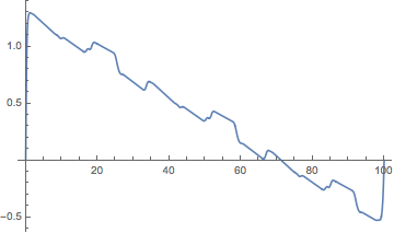
swayOfTime[t_] := sway[swayTimeCoordinate[t]/100][[2]] Plot[swayOfTime[t], {t, 0, 10}] 
Visualize phrases and their relationship to movement with a tooltip and colored rectangles:
phraseGraphics = BlockMap[ Apply[ Function[{currentAnchor, nextAnchor}, With[ {phraseStart = currentAnchor["PickupBeat"], phraseEnd = nextAnchor["PickupBeat"] - currentAnchor["BeatLength"]}, {Switch[currentAnchor["PhraseName"], "O Christmas Tree", Opacity[0.25, Gray], "Your boughs so green in summertime", Opacity[0.25, Darker@Green], _, Black], Tooltip[ Polygon[ {{phraseStart, -10}, {phraseStart, 10}, {phraseEnd, 10}, {phraseEnd, -10}}], Grid[{{currentAnchor["PhraseName"], SpanFromLeft}, {"Phrase Start:", phraseStart}, {"Phrase End:", phraseEnd} }]]}]]], Append[anchorData0, <|"PickupBeat" -> lastBeat + meanBeatLength|>], 2, 1]; Show[swayControlPointPlot, ParametricPlot[sway[t], {t, 0, Last[measureBeats]}, ImageSize -> Full, PlotPoints -> 800, AspectRatio -> 1/8, PlotTheme -> "Detailed", PlotRangePadding -> Scaled[.02]], Prolog -> phraseGraphics] 
Movement Conductor
The conductor performs a simple periodic movement, synchronized with the music.
threePatternPoints = {{0, -1}, {-1, -0}, {0, 1}}; threePatternBackground = ListPlot[ MapIndexed[ Callout[#1, StringTemplate["Beat #`` @ ``"][First@#2, #1], Left] &, threePatternPoints], PlotTheme -> "Minimal", Axes -> False, AspectRatio -> 1, PlotStyle -> Directive[Black, PointSize[0.025]], PlotRange -> {{-2, 0.75}, {-1.5, 1.5}}]; conductorControlTimes = swayControlPoints[[All, 1]]; (* basic conductor control points for interpolation *) conductorControlPoints = MapIndexed[{conductorControlTimes[[First[#2]]], #1} &, Join @@ ConstantArray[RotateRight[threePatternPoints, 1], Floor@(Length[conductorControlTimes]/3)]]; (* the shape is okay, but not perfect *) conductor = Interpolation[conductorControlPoints]; (* adding pauses before/after the beat improves the shape of the curves and makes the beats more obvious *) conductorControlPointsWithPauses = Join @@ ({# - {meanBeatLength/8., -0.15* Normalize[ Mean[threePatternPoints] - #[[ 2]]]}, #, # + {meanBeatLength/8., 0.15*Normalize[ Mean[threePatternPoints] - #[[ 2]]]}} & /@ conductorControlPoints); Interpolation.
conductorWithPauses = Interpolation[conductorControlPointsWithPauses, InterpolationOrder -> 5]; .
Manipulate[ Show[threePatternBackground, ParametricPlot[ conductorWithPauses[t], {t, Max[firstBeat,(*tmax-2*meanBeatLength*)0], tmax}, PerformanceGoal -> "Quality"], Epilog -> {Red, PointSize[Large], Point[conductorWithPauses[tmax]]}, ImageSize -> Large], {{tmax, lastBeat, "t"}, firstBeat + 0.0001, lastBeat, Appearance -> "Labeled"}, SaveDefinitions -> True] 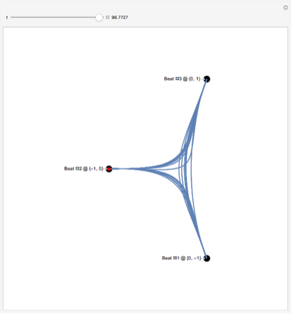
. : , — .
1
2D : : :
δDelay = 0.3; voiceστ[j_][time_] := If[0 < time < tMax,(* smoothing factor *) Sin[Pi time/tMax]^0.25 {voiceFunction[j][1. time] - voiceFunction[j][time - δDelay], voiceFunction[j][1. time]}, {0, 0}] ParametricPlot[voiceστ[1][t], {t, 0, tMax}, AspectRatio -> 1, PlotRange -> All, Frame -> True, Axes -> False, PlotStyle -> Thickness[0.002]] 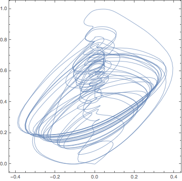
Option 2
2D : : :
value = -1; interpolateDance[{{t1_, t2_}, {t3_, t4_}}, t_] := With[{y1 = value, y2 = value = -value}, {{y1, t1 < t < t2}, {((y1 - y2) t - (t3 y1 - t2 y2))/(t2 - t3), t2 < t < t3}}]; dancingPositionPiecewise[notes : {__SoundNote}] := With[{noteTimes = Cases[notes, SoundNote[_, times : {startTime_, endTime_}, ___] :> times]}, value = -1; Quiet[Piecewise[ DeleteDuplicatesBy[ Join @@ BlockMap[interpolateDance[#, t] &, noteTimes, 2, 1], Last], 0] ]]; tEnd = Max[voices[[All, All, 2]]]; dancingPositions = dancingPositionPiecewise /@ voices; Plot[Evaluate[KeyValueMap[Legended[#2, #1] &, dancingPositions]], {t, 0, 50}, PlotRangePadding -> Scaled[.05], PlotRange -> {All, {-1, 1}}, ImageSize -> Large, PlotTheme -> "Detailed", PlotLegends -> None] 
dancingPositionPiecewiseList = Normal[dancingPositions][[All, 2]]; bsp = BSplineFunction[ Table[Evaluate[{t, dancingPositionPiecewiseList[[2]]}], {t, 0, 100, 0.2}]] ParametricPlot[bsp[t], {t, 0, 1}, AspectRatio -> 1/4, PlotPoints -> 2000] 
Do[voiceIF[j] = BSplineFunction[ Table[Evaluate[{t, dancingPositionPiecewiseList[[j]]}], {t, 0, 100, 0.2}]], {j, 4}] Do[With[{j = j}, voiceTimeCoordinate[j] = Interpolation[Table[{t, voiceIF[j][t/100][[1]]}, {t, 0, 100, 0.1}], InterpolationOrder -> 1]], {j, 4}] σ-τ [-1,1] * [- 1,1].
Clear[voiceστ]; voiceστ[j_][time_] := If[0 < time < tMax,(* smoothing factor *) Sin[Pi time/tMax]^0.25* {sway[swayTimeCoordinate[time]/tMax][[2]], voiceIF[j][voiceTimeCoordinate[j][time]/tMax][[2]]}, {0, 0}] Table[ListPlot[Table[ voiceστ[j][t], {t, 0, 105, 0.01}], Joined -> True, AspectRatio -> 1, PlotStyle -> Thickness[0.002]], {j, 4}] 
() . (, ) . , , , voiceστ [j] [time].
.
Clear[r, ρ, R, X, Y, Z] R[t_] := {X[t], Y[t], Z[t]} r[t_] := R[t] + L {Cos[ϕ[t]] Sin[θ[t]], Sin[ϕ[t]] Sin[θ[t]], -Cos[θ[t]]} ℒ = 1/2 r'[t].r'[t] - gr[t][[3]] -g (-L Cos[θ[t]] + Z[t]) + 1/2 ((Derivative[1][Z][t] + L Sin[θ[t]] Derivative[1][θ][t])^2 + (Derivative[ 1][Y][t] + L Cos[θ[t]] Sin[ϕ[t]] Derivative[1][θ][t] + L Cos[ϕ[t]] Sin[θ[t]] Derivative[1][ϕ][ t])^2 + (Derivative[1][X][t] + L Cos[θ[t]] Cos[ϕ[t]] Derivative[1][θ][t] — L Sin[θ[t]] Sin[ϕ[t]] Derivative[1][ϕ][t])^2)
ℱ .
ℱ = 1/2 (\[ScriptF]ϕ ϕ'[t]^2 + \[ScriptF]θ θ'[t]^2); eoms = {D[D[ℒ, ϕ'[t]], t] - D[ℒ, ϕ[t]] == -D[ℱ, ϕ'[t]], D[D[ℒ, θ'[t]], t] - D[ℒ, θ[t]] == -D[ℱ, θ'[ t]]} // Simplify {([ScriptF]ϕ + L^2 Sin[2 θ[t]] Derivative[1][θ][t]) Derivative[ 1][ϕ][t] + L Sin[θ[t]] (-Sinϕ[t]t] + Cos[ϕ[t][t] + L Sinθ[t][t]) == 0, [ScriptF]θ Derivative[1][θ][t] + L (g Sin[θ[t]] — L Cos[θ[t]] Sin[θ[t]] Derivative[1][ϕ][t]^2 + Cos[θ[t]] Cosϕ[t]t] + Cos[θ[t]] Sin[ϕ[t]t] + Sin[θ[t][t] + L (θ^′′)[t]) == 0}
, , [ScriptF] φ, [ScriptF] θ.
paramRules = { g -> 10, L -> 1, \[ScriptF]ϕ -> 1, \[ScriptF]θ -> 1}; In[126]:= X[t_] := If[2 Pi < t < 4 Pi, 8 Cos[t], 8]; Y[t_] := If[2 Pi < t < 4 Pi, 4 Sin[t], 0]; Z[t_] := 0; nds = NDSolve[{eoms /. paramRules, ϕ[0] == 1, ϕ'[0] == 0, θ[0] == 0.001, θ'[0] == 0}, {ϕ, θ}, {t, 0, 20}, PrecisionGoal -> 3, AccuracyGoal -> 3] 
Plot[Evaluate[{\[Phi][t], \[Theta][t]} /. nds[[1]]], {t, 0, nds[[1, 2, 2, 1, 1, 2]]}, PlotRange -> All] 
Graphics3D[ Table[With[{P = r[t] - R[t] /. nds[[1]] /. paramRules}, {Black, Sphere[{0, 0, 0}, 0.02], Gray, Cylinder[{{0, 0, 0}, P}, 0.005], Darker[Blue], Sphere[P, 0.02]}], {t, 0, 20, 0.05}], PlotRange -> All] 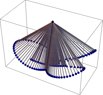
δ τ , .
branchToVoice = Association[ Flatten[Function[{v, bs}, (# -> v) & /@ bs] @@@ Normal[voiceBranches]]] <|2 -> 1, 9 -> 1, 14 -> 1, 17 -> 1, 19 -> 1, 24 -> 1, 27 -> 1, 3 -> 2, 13 -> 2, 15 -> 2, 16 -> 2, 21 -> 2, 26 -> 2, 1 -> 3, 4 -> 3, 5 -> 3,
12 -> 3, 18 -> 3, 20 -> 3, 6 -> 4, 8 -> 4, 10 -> 4, 11 -> 4, 22 -> 4, 23 -> 4, 25 -> 4|>
tValues = Table[1. t , {t, -5, 110, 0.1}]; Do[στValues = Table[voiceστ[j][t] , {t, -5, 110, 0.1}]; ifσ[j] = Interpolation[ Transpose[{tValues, στValues[[All, 1]]}]]; ifτ[j] = Interpolation[ Transpose[{tValues, στValues[[All, 2]]}]], {j, 4}] , . , ( ).
( ) .
changeTimeList = {17.6, 42.2, 66.8, 83.1}; loudness[t_] := With[{λ1 = 0.2, λ2 = 0.8, δt = 1.5}, Which[t <= changeTimeList[[3]] - δt, λ1, changeTimeList[[3]] - δt <= t <= changeTimeList[[3]] + δt, λ1 + (λ2 - 1 λ1) (1 - Cos[Pi (t - (changeTimeList[[ 3]] - δt))/(2 δt)])/2, changeTimeList[[3]] + δt <= t <= changeTimeList[[4]] - δt , λ2, changeTimeList[[4]] - δt <= t <= changeTimeList[[4]] + δt, λ1 + (λ2 - 1 λ1) (1 + Cos[Pi (t - (changeTimeList[[ 4]] - δt))/(2 δt)])/2, t >= changeTimeList[[3]] + 1.5, λ1] ] Plot[loudness[t], {t, 1, 100}, AxesOrigin -> {0, 0}, PlotRange -> All] 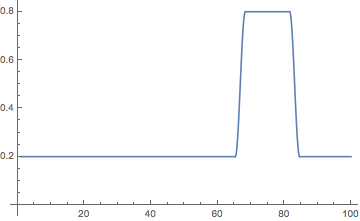
Off[General::stop]; SeedRandom[111]; Monitor[ Do[ branchEnd[j, {σ_, τ_}] = branchOnStemEndPoint[ allBranches[[j]], {τ, σ}]; If[j =!= conductorBranch, With[{v = branchToVoice[j]}, tipPosition[t_] = branchEnd[j, loudness[t] {ifσ[v][t], ifτ[v][t]}]]; {X[t_], Y[t_], Z[t_] } = tipPosition[t]; paramRules = { g -> 20, L -> 1, \[ScriptF]ϕ -> 1, \[ScriptF]θ -> 1}; While[ Check[ pendulumϕθ[j][t_] = NDSolveValue[{eoms /. paramRules, ϕ[0] == RandomReal[{-Pi, Pi}], ϕ'[0] == 0.01 RandomReal[{-1, 1}], θ[0] == 0.01 RandomReal[{-1, 1}], θ'[0] == 0.01 RandomReal[{-1, 1}]}, {ϕ[t], θ[t]}, {t, 0, 105}, PrecisionGoal -> 4, AccuracyGoal -> 4, MaxStepSize -> 0.01, MaxSteps -> 100000, Method -> "BDF"]; False, True]] // Quiet], {j, Length[allBranches]}], j] . .
Plot[pendulum\[Phi]\[Theta][51][t][[2]], {t, 0, 105}, AspectRatio -> 1/4, PlotRange -> All] 
.
SeedRandom[11]; Do[randomColor[j] = RandomColor[]; randomAngle[j] = RandomReal[{-Pi/2, Pi/2}], {j, Length[allBranches]}] .
conductorστ[t_] := Piecewise[ {{{0, 0}, t <= firstBeat/ 2}, {(t - firstBeat/2)/(firstBeat/2) conductorControlPointsWithPauses[[ 1, 2]], firstBeat/2 < t <= firstBeat}, {conductorWithPauses[t], firstBeat < t <= lastBeat}, {(tMax - t)/(tMax - lastBeat) conductorControlPointsWithPauses[[-1, 2]], lastBeat < t < tMax}, {{0, 0}, t >= tMax}}] .
ListPlot[{Table[{t, conductorστ[t][[1]]}, {t, -1, 3, 0.01}], Table[{t, conductorστ[t][[2]]}, {t, -1, 3, 0.01}]}, PlotRange -> All, Joined -> True] 
With[{animationType = 2}, scalefactors[1][t_] := Switch[animationType, 1, {0.8, 1} , 2, loudness[t]]; scalefactors[2][t_] := Switch[animationType, 1, {1, 1} , 2, loudness[t]]; scalefactors[3][t_] := Switch[animationType, 1, {1, 1} , 2, loudness[t]]; scalefactors[4][t_] := Switch[animationType, 1, {1, 1} , 2, loudness[t]] ] christmasTreeWithSwingingOrnaments[t_, conductorEnhancementFactor : fc_, conductorCandleAngle : ωc_, topRotationAngle : ω_, opts___] := Graphics3D[{{Darker[Brown], stem}, (* first voice *) branchOnStemWithBall[allBranches[[#]], scalefactors[1][t] voiceστ[1][t], Darker[Yellow, -0.1], If[t < 0, {0, 0}, pendulumϕθ[#][t]]] & /@ voiceBranches[[1]], (* second voice *) branchOnStemWithBall[allBranches[[#]], scalefactors[2] [t] voiceστ[2][t], Blend[{Red, Pink}], If[t < 0, {0, 0}, pendulumϕθ[#][t]]] & /@ voiceBranches[[2]], (* third voice *) branchOnStemWithFiveStar[allBranches[[#]], scalefactors[3][t] voiceστ[3][t], randomColor[#], Pi/4, If[t < 0, {0, 0}, pendulumϕθ[#][t]]] & /@ voiceBranches[[3]], (* fourth voice *) branchOnStemWithCandle[#, scalefactors[4][t] voiceστ[4][t], Directive[White, Glow[GrayLevel[0.3]], Specularity[Yellow, 20]], 0] & /@ allBranches[[voiceBranches[[4]]]], (* conductor *) branchOnStemWithCandle[ allBranches[[conductorBranch]] {1, 1, 1 + fc}, conductorστ[t], Directive[Red, Glow[GrayLevel[0.1]], Specularity[Yellow, 20]], ωc], Rotate[top, ω, {0, 0, 1}] }, opts, ViewPoint -> {2.8, 1.79, 0.1}, PlotRange -> {{-8, 8}, {-8, 8}, {-2, 15}}, Background -> RGBColor[0.998, 1., 0.867] ] , .
Show[christmasTreeWithSwingingOrnaments[70, 0.5, 0.8, 2], PlotRange -> All, Boxed -> False] 
!
() . , 3D-, . , PDE (http://psoup.math.wisc.edu/papers/h3l.pdf), , , .
(2D)
- « - ». , hex snowflake.
ReleaseHold /@ (MakeExpression[#[[1]], StandardForm] & /@ Take[Cases[ Import["http://demonstrations.wolfram.com/downloadauthornb.cgi?\ name=SnowflakeLikePatterns"], Cell[_, "Input", ___], ∞], 2]); makeSnowflake[rule_, steps_] := Polygon[hex[#] & /@ Select[Position[Reverse[CellularAutomaton[ {snowflakes[[ rule]], {2, {{0, 2, 2}, {2, 1, 2}, {2, 2, 0}}}, {1, 1}}, {{{1}}, 0}, {{{steps}}, {-steps, steps}, {-steps, steps}}]], 0], -steps - 1 < -#[[1]] + #[[2]] < steps + 1 &]] SeedRandom[33]; Table[Graphics[{Darker[Blue], makeSnowflake[RandomInteger[{1, 3888}], RandomInteger[{10, 60}]]}], {4}] 
, , . , .
denseFlakeQ[mr_MeshRegion] := With[{c = RegionCentroid[mr], pts = MeshCoordinates[mr]}, ( Divide @@ MinMax[EuclideanDistance[c, #] & /@ pts]) < 1/3] randomSnowflakes[] := Module[{sf}, While[(sf = Module[{}, TimeConstrained[ hexagons = makeSnowflake[RandomInteger[{1, 3888}], RandomInteger[{10, 60}]]; (Select[ConnectedMeshComponents[DiscretizeRegion[hexagons]], (Area[#] > 120 && Perimeter[#]/Area[#] < 2 && denseFlakeQ[#]) &] /. \ _ConnectedMeshComponents :> {}) // Quiet, 20, {}]]) === {}]; sf] randomSnowflakes[n_] := Take[NestWhile[Join[#, randomSnowflakes[]] &, {}, Length[#] < n &], n] SeedRandom[22]; randomSnowflakes[4] 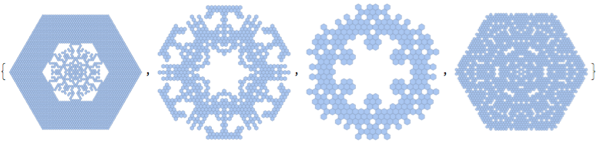
normalizeFlake[mr_MeshRegion] := Module[{coords, center, coords1, size, coords2}, coords = MeshCoordinates[mr]; center = Mean[coords]; coords1 = (# - center) & /@ coords; size = Max[Norm /@ coords1]; coords2 = coords1/size; GraphicsComplex[coords2, {EdgeForm[], MeshCells[mr, 2]}]] .

(3D)
2D , , 3D .
make3DFlake[flake2D_] := Module[{grc, reg, boundary, h, bc, rb, polys, pts}, grc = flake2D[[1]]; reg = MeshRegion @@ (grc /. _EdgeForm :> Nothing); boundary = (MeshPrimitives[#, 1] &@RegionBoundary[reg])[[All, 1]]; h = RandomReal[{0.05, 0.15}]; bc = Join[#1, Reverse[#2]] & @@@ Transpose[{Map[Append[#, 0] &, boundary, {-2}], Map[Append[#, h] &, boundary, {-2}]}]; rb = RegionBoundary[reg]; boundary = (MeshCells[#, 1] &@rb)[[All, 1]]; polys = Polygon[Join[#1, Reverse[#2]] & @@@ Transpose[{boundary, boundary + Max[boundary]}]]; pts = Join[Append[#, 0] & /@ MeshCoordinates[rb], Append[#, h] & /@ MeshCoordinates[rb]]; {GraphicsComplex[Developer`ToPackedArray[pts], polys], MapAt[Developer`ToPackedArray[Append[#, 0]] & /@ # &, flake2D[[1]], 1], MapAt[Developer`ToPackedArray[Append[#, h]] & /@ # &, flake2D[[1]], 1]} ] listOfSnowflakes3D = make3DFlake /@ listOfSnowflakes; Graphics3D[{EdgeForm[], #}, Boxed -> False, Method -> {"ShrinkWrap" -> True}, ImageSize -> 120, Lighting -> {{"Ambient", Hue[.58, .5, 1]}, {"Directional", GrayLevel[.3], ImageScaled[{1, 1, 0}]}}] & /@ listOfSnowflakes3D 
1994 . , , .
Manipulate[ Module[{eqs, nds, tmax, g = 10, α, sign, V, x, y, u, v, θ, ω, kpar = kperp/f, ρ = 10^ρexp}, α = ArcTan[u[t], v[t]]; sign = Piecewise[{{1, (v[t] < 0 && 0 <= α + θ[t] <= Pi) || (v[t] > 0 && -Pi <= α + θ[t] <= 0)}}, -1]; V = Sqrt[u[t]^2 + v[t]^2]; eqs = {D[x[t], t] == u[t], D[y[t], t] == v[t], D[u[t], t] == -(kperp Sin[θ[t]]^2 + kpar Cos[θ[t]]^2) u[ t] + (kperp - kpar) Sin[θ[ t]] Cos[θ[t]] v[t] - sign Pi ρ V^2 Cos[α + θ[t]] Cos[α], D[v[t], t] == -(kperp Cos[θ[t]]^2 + kpar Sin[θ[t]]^2) v[ t] + (kperp - kpar) Sin[θ[ t]] Cos[θ[t]] u[t] + sign Pi ρ V^2 Cos[α + θ[ t]] Sin[α] - g, D[ω[t], t] == -kperp ω[ t] - (3 Pi ρ V^2/l) Cos[α + θ[ t]] Sin[α + θ[t]], D[θ[t], t] == ω[t]} /. kpar -> kperp/f; nds = NDSolve[ Join[eqs, {x[0] == 0, y[0] == 0, u[0] == 0, v[0] == 0.01, ω[0] == 0, θ[0] == θ0}], {x, y, u, v, θ, ω}, {t, 0, T}, MaxSteps -> 2000] // Quiet; tmax = nds[[1, 2, 2, 1, 1, 2]]; Graphics[{Thickness[0.002], Gray, Table[Evaluate[ Line[{{x[t], y[t]} - l/2 {Cos[θ[t]], Sin[θ[t]]}, {x[t], y[t]} + l/2 {Cos[θ[t]], Sin[θ[t]]}}] /. nds[[1]]], {t, 0, tmax, tmax/n}], Blue, Line[Table[ Evaluate[{x[t], y[t]} /. nds[[1]]], {t, 0, tmax, tmax/200}]]}, AspectRatio -> ar, Frame -> True, PlotRange -> All]], "system parameters", {{kperp, 5.1, Subscript["k", "∟"]}, 0.01, 10, Appearance -> "Labeled"}, {{f, 145, Row[{Subscript["k", "∟"], "/", Subscript["k", "∥"]}]}, 0.01, 200, Appearance -> "Labeled"}, {{ρexp, -0.45, Log["ρ"]}, -3, 1, Appearance -> "Labeled"}, {{l, 0.63}, 0.01, 10, Appearance -> "Labeled"} , Delimiter, "fall parameters", {{θ0, 1, Subscript["θ", "0"]}, -Pi, Pi, Appearance -> "Labeled"}, {{T, 2, "falling time"}, 0, 10, Appearance -> "Labeled"} , Delimiter, "plot", {{ar, 1, "aspect ratio"}, {1, Automatic}}, {{n, 200, "snapshots"}, 2, 500, 1}] 
, . / , .
, .
randomParametrizedRotationMatrix[n_, τ_] := Function @@ {τ, Module[{phi, s, c}, Do[phi[i] = Sum[RandomReal[{-1, 1}] Sin[ RandomReal[{0, n}] τ + 2 Pi RandomReal[]], {n}]; {c[i], s[i]} = {Cos[phi[i]], Sin[phi[i]]}, {i, 3}]; {{c[1], s[1], 0}, {-s[1], c[1], 0}, {0, 0, 1}}. {{c[2], 0, s[2]}, {0, 1, 0}, {-s[2], 0, c[2]}}. {{1, 0, 0}, {0, c[3], s[3]}, {0, -s[3], c[3]}}]}; randomParametrizedPathFunction := Function[t, Evaluate[{RandomReal[{-5, 5}] + Sum[RandomReal[{-1, 1}]/# Cos[2 Pi # t] &[ RandomReal[{1, 4}]], {k, 5}], RandomReal[{-5, 5}] + Sum[RandomReal[{-1, 1}]/# Cos[2 Pi # t] &[ RandomReal[{1, 4}]], {k, 5}], RandomReal[{2, 12}] - RandomReal[{1.5, 2.5}] t}]] SeedRandom[55]; Do[rotMat[j] = randomParametrizedRotationMatrix[3, τ]; trans[j] = randomParametrizedPathFunction; snowflakeColor[ j] = {{"Ambient", Hue[RandomReal[{0.55, 0.6}], RandomReal[{0.48, 0.52}], RandomReal[{0.95, 1}]]}, {"Directional", GrayLevel[RandomReal[{0.28, 0.32}]], ImageScaled[{1, 1, 0}]}}, {j, Length[listOfSnowflakes]}] fallingSnowflake[flake_, {t_, ℛ_}] := flake /. GraphicsComplex[cs_, rest__] :> GraphicsComplex[(ℛ.# + t) & /@ cs, rest] Manipulate[ Graphics3D[{EdgeForm[], Table[{Lighting -> snowflakeColor[k], fallingSnowflake[ listOfSnowflakes3D[[k]], {trans[k][t], rotMat[k][t]}]}, {k, Length[listOfSnowflakes3D]}] }, PlotRange -> 6, ViewPoint -> {0, -10, 0}, ImageSize -> 400], {{t, 3.2}, -5, 20}] 
.
, , . . , . , , . 24 .
conductorBranchMaxfactor = 0.5; conductorBranchLength[t_] := conductorBranchMaxfactor* Which[t < -3, 0, -3 < t <= 0, (t + 3)/3., 0 <= t <= tMax, 1, tMax < t < tMax + 3, (1 - (t - tMax)/3), True, 0]; topRotation[t_] := Which[t < -3 || t > tMax + 3, 0, True, (1. - Cos[(t + 3)/(tMax + 6)]) 20 2 Pi]; viewPoint[t_] := With[{vp = {2.8, 1.79, 0.1}}, Which[t < changeTimeList[[1]] || t > changeTimeList[[2]], vp, changeTimeList[[1]] <= t <= changeTimeList[[2]], Module[{t0 = changeTimeList[[1]], Δt = changeTimeList[[2]] - changeTimeList[[1]], ωvp}, ωvp = -Pi (1 - Cos[ Pi (t - t0)/Δt]); {{Cos[ωvp], Sin[ωvp], 0}, {-Sin[ωvp], Cos[ωvp], 0}, {0, 0, 1}}.vp + {0, 0, 2 Sin[Pi (t - t0)/Δt]^4 }]]] ParametricPlot3D[ viewPoint[t], {t, changeTimeList[[1]], changeTimeList[[2]]}, BoxRatios -> {1, 1, 1}] 
animationFrame[t_] := Show[christmasTreeWithSwingingOrnaments[t, conductorBranchLength[t], 1.4 conductorBranchLength[t], topRotation[t]], Background -> None, Boxed -> False, SphericalRegion -> True, ViewPoint -> viewPoint[t]] , :
animationFrame[35] 
framesPerSecond = 24; animationFrameDirectory = "/Users/mtrott/Desktop/ConductingChristmasTreeAnimationFrames/"; Monitor[ Do[ With[{t = -3 + 1/framesPerSecond (frame - 1)}, gr = animationFrame[t]; Export[animationFrameDirectory <> IntegerString[frame, 10, 4] <> ".png", gr, ImageSize -> 1800, Background -> None] ], {frame, 1, framesPerSecond (100 + 2 3)}], Row[{frame, " | ", Round[MemoryInUse[]/1024^2], "\[ThinSpace]MB" }] ] (, Adobe After Effects) , .
info-russia@wolfram.com
Mathematica
Wolfram|One
Source: https://habr.com/ru/post/345358/
All Articles