Ratings of car brands: an example of analyzing variables with multiple response

In questionnaire marketing research quite often there are questions in which respondents can choose several suitable options from the list of possible answers (check all that apply questions). Answers of respondents to such questions are set by variables with multiple response (multiple-response variables). The appropriate statistical methods for working with multiple-response variables are not widely known. In this article, we consider the analysis of such variables on the example of data on car ratings.

Data

This is a typical example of a questionnaire that allows multiple answers.

Customer Satisfaction Survey Template. Source: Survey Monkey

We will use data on car ratings in this article (Van Gysel 2011). They are freely distributable and are included in the plfm R-package. These data should be perceived only as an object for the demonstration of mathematical methods and visualization tools. One should not assume that the results were obtained on the basis of a full-fledged representative survey of any group.

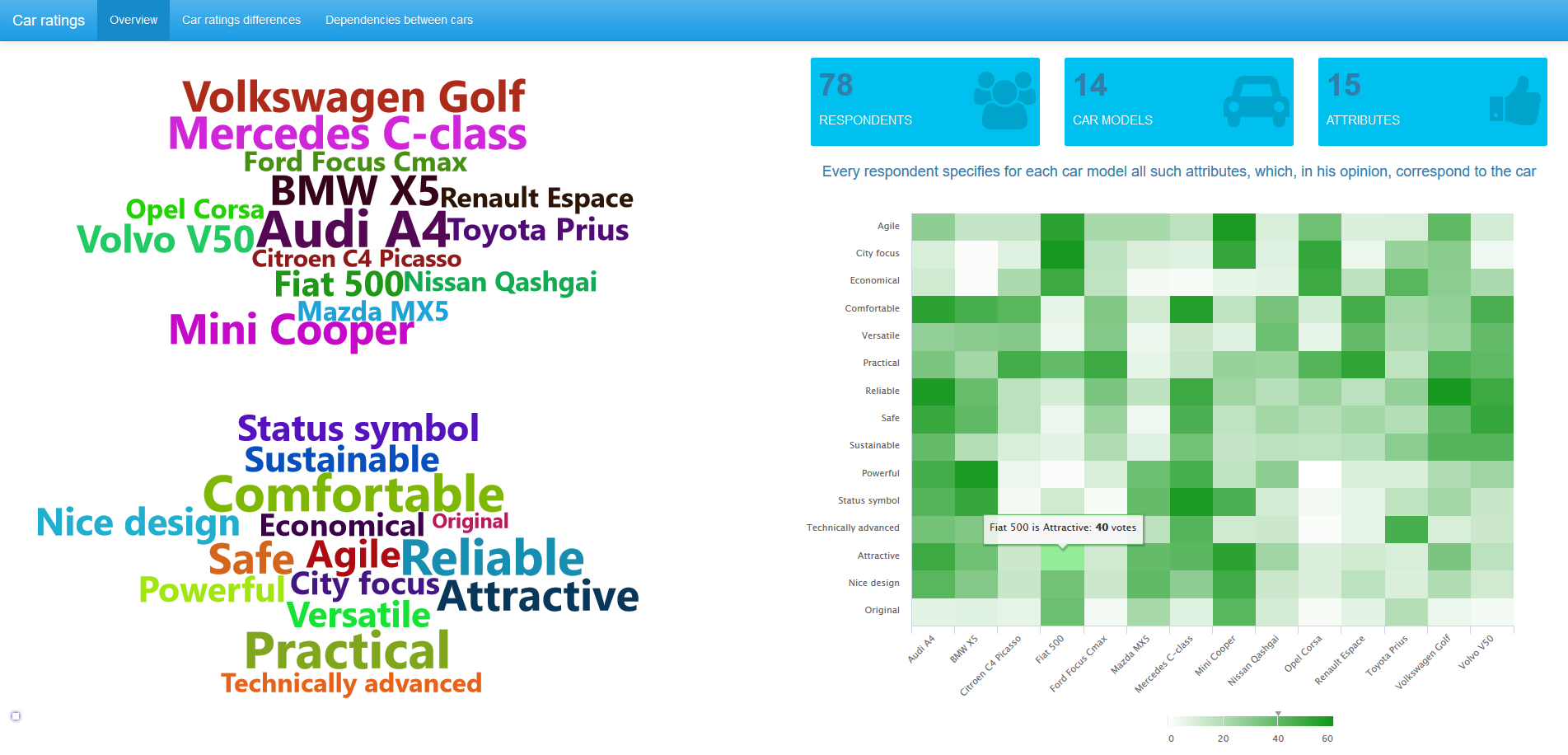
The header image provides an overview of the data, all click-through images open in full size. We see that 78 respondents participated in the survey. The survey questionnaire found out opinions on 14 car brands. For each of them, the respondents noted those characteristics (from the proposed list with 15 names) to which the car corresponds. The picture above shows that 40 respondents believe that the Fiat 500 is an attractive car.

Rating Comparison

To compare the ratings on the characteristics between the two cars, the well-known McNemar test, or rather its McNemar mid-p test, is used. This test analyzes paired observations. The mid-p correction allows working with small samples and is less conservative than the exact binomial test. Details can be found, for example, in this article (Fagerland, Lydersen, and Laake 2013).

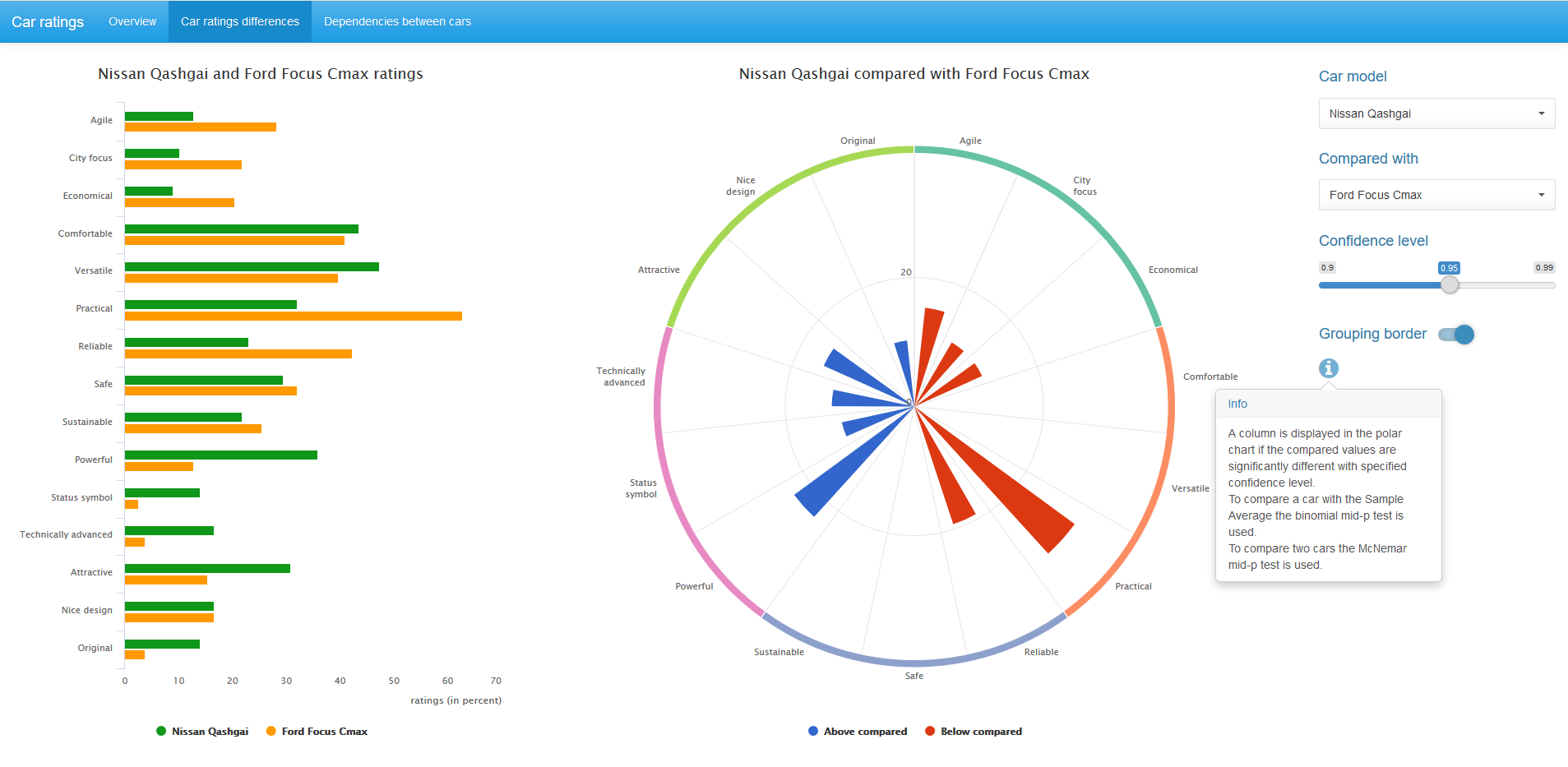
The diagram in the center displays only statistically significant, for a given confidence level, differences in ratings between a pair of compared cars. Blue color corresponds to a higher rating value for the first car, red - for the second.

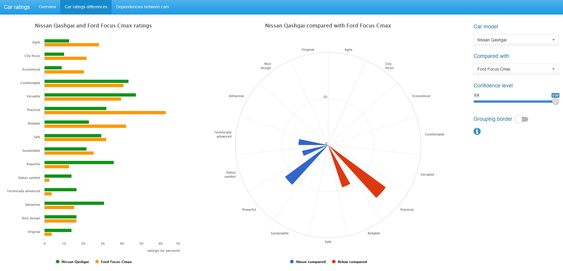
We can change the confidence level value and, if desired, remove the grouping border on the diagram.

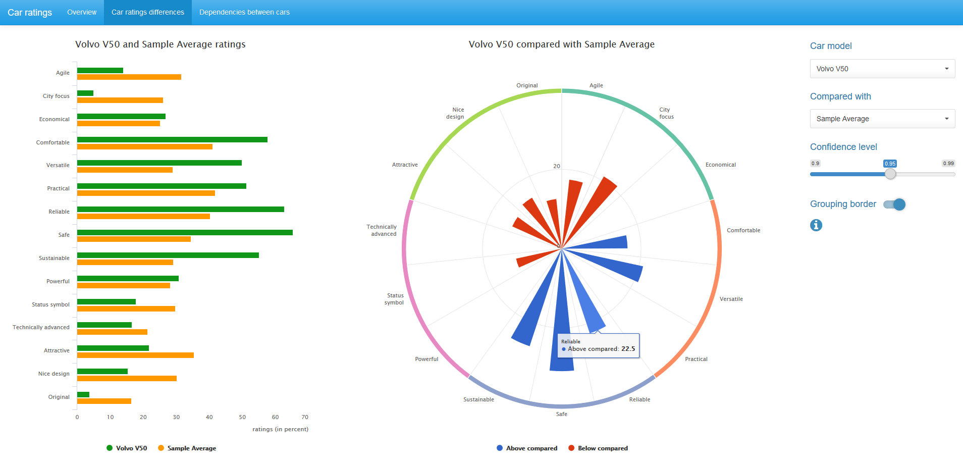
You can also compare the values ​​of the ratings of the car with the average selection ratings for all 14 cars. In this case, use the binomial mid-p test.

Both the McNemar mid-p test and the binomial mid-p test are available in the exact2x2 R-package, but can be easily implemented with the basic R tools.

Dependence between two multiple-response variables

The task is as follows: we have chosen a set of characteristics and an arbitrary pair of car models. Is it possible to assert that the distribution of respondent answers for these cars is independent? In other words, we have no reason to believe that there is some statistical relationship in the rating of these two brands in a given set of characteristics.

For example, consider the following 8x8 table:

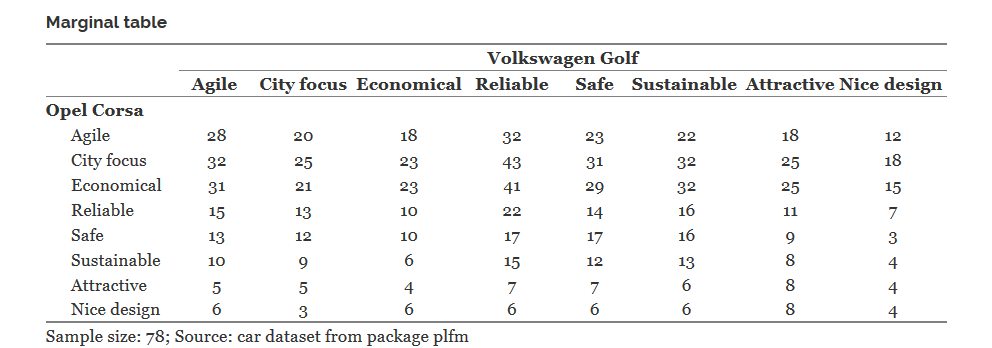
In it, the value of the cell, say Opel Corsa | Economical - Volkswagen Golf | Relible, equal to 41, means that exactly 41 respondents indicated that the Opel Corsa is an economical car and the Volkswagen Golf is reliable.

If both the Opel Corsa and Volkswagen Golf were single-response variables, this table would set the joint distribution of these variables. Then we could apply a chi-square test to this table to check the independence of this pair of variables. But we have a completely different case, and according to this table, for example, it is even unclear how many respondents believe that the Opel Corsa is an economical car.

For each cell of this marginal table sits a 2x2 table, which determines the distribution in a separate pair of selected characteristics. These 8 tables for the diagonal cells of the marginal table were used in McNemar tests for this pair of cars.

But this set of all 64 tables is not enough to specify the joint distribution of two multiple-response variables with 8 categories each. In general, this will require a table size $$$2 ^ 8 \ times 2 ^ 8$. So, the sum of 64 chi-squares of statistics found for 2x2 tables, due to the dependence of the observations (not variables) in the input data, is not a value $$$\ chi_ {64}$distribution. Information from the table $$$2 ^ 8 \ times 2 ^ 8$allow you to find a second-order Rao-Scott amendment and apply it to the sum of these 64 chi-square values. Details and formulation of the criterion of independence can be found in the article (Bilder and Loughin 2004).

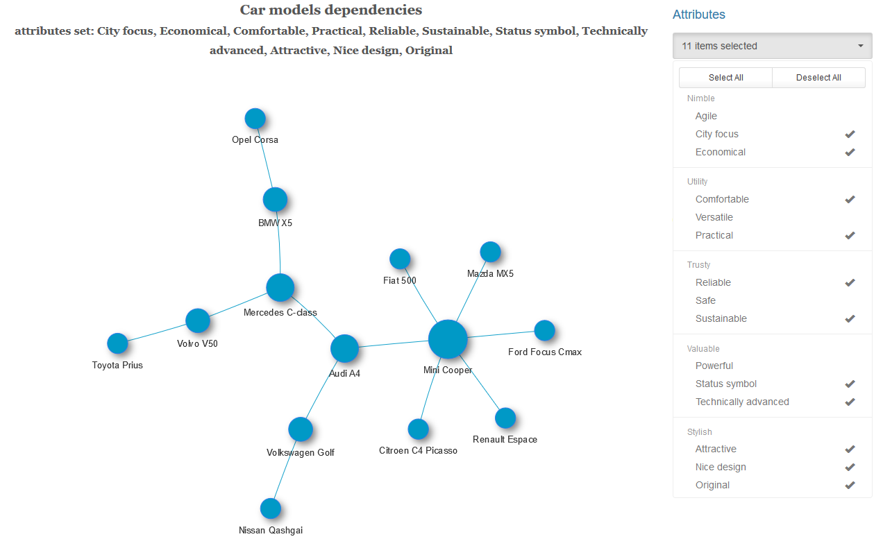
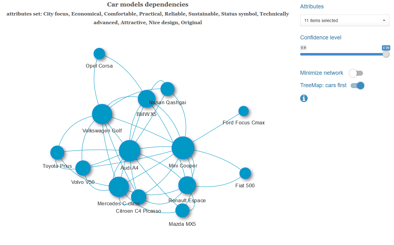
For each pair of vehicles with a given set of characteristics and at the chosen level of significance, we check the hypothesis of independence of these variables. If the independence hypothesis is rejected, we connect this pair of cars with an edge with a weight equal to the p-value of the obtained Rao-Scott statistics. We obtain a weighted graph, to which we optionally apply an algorithm for finding the minimum spanning tree (for each connected component of the graph). That is, we leave the minimum possible number of the strongest bonds.

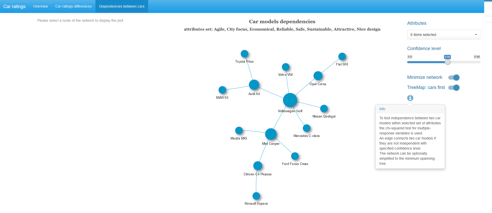
When you click on the picture, it will open in full size.
Almost half of the cars in the resulting graph is the strongest dependence observed with the Volkswagen Golf.

If a vertex of the graph is selected, then in addition a treemap of the chi-squared 2x2 statistics table with pairs of characteristics for adjacent vertices is displayed.

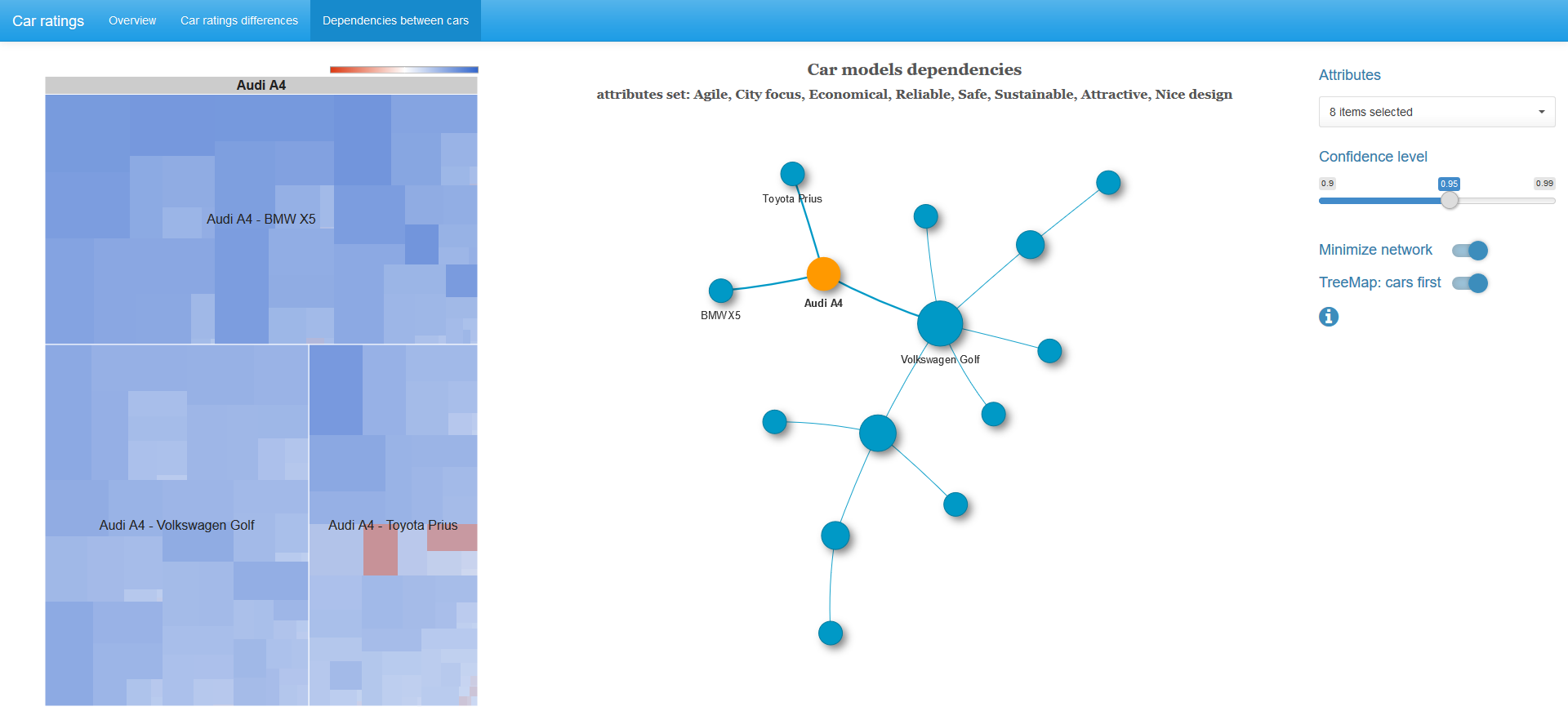
The cell size is proportional to the chi-square statistic, the color is determined by the logarithm of the odds ratio: the blue spectrum is positive values, the white color is zero, the red spectrum is negative values. The color scale is not symmetrical, that is, the left border in absolute value does not necessarily coincide with the right edge of the scale.

Below are examples of a minimum spanning tree with a different set of characteristics and a graph with a full set of links.

Calculate and run the application

The approach proposed in (Bilder and Loughin 2004) is implemented in the R-package MRCV . However, for the above 8x8 marginal table, the independence check function for these variables from this library returns an error: cannot allocate vector of size 32.0 Gb . The reason is that in the process of calculating order matrices arise $$$2 ^ {16} \ times 2 ^ {16}$.

An approach was proposed in which the implementation of this test in R does not require such a large amount of memory and is much more productive. For comparison, the calculation of the complete graph with 14 vertices and 7 characteristics in the MRCV package will take more than 30 minutes. In an improved implementation, this calculation is performed for about 1 second. In this pdf you can find the details of this calculation method. Source code and performance tests are available on github .

You can start this shiny application yourself by running the R commands.

 library(shiny) runGitHub("BrandsAnalysis", "e-chankov") 

Make sure you have installed

 #### shiny libraries library(shiny) # version 1.0.5 library(shinythemes) # version 1.1.1 library(shinydashboard) # version 0.6.1 library(shinyBS) # version 0.61 library(shinyWidgets) # version 0.3.6 #### libraries for visualization library(wordcloud2) # version 0.2.0 library(highcharter) # version 0.5.0 library(googleVis) # version 0.6.2 library(visNetwork) # version 2.0.1 library(RColorBrewer) # version 1.1-2 #### data munging libraries library(data.table) # version 1.10.4 library(checkmate) # version 1.8.4 library(Matrix) # version 1.2-11 library(igraph) # version 1.1.2 library(stringi) # version 1.1.5 

Input data is read from a text file. The application can be used to analyze data from surveys about any brands with its own set of characteristics. Input requirements can be found in the application description .

Literature

Bilder, C., and T. Loughin. 2004. “Testing for Marginal Independence Between Two Categorical Variables with Multiple Responses.” Biometrics 60 (1): 241–48. http://dx.doi.org/10.1111/j.0006-341X.2004.00147.x .

Fagerland, Morten W., Stian Lydersen, and Petter Laake. 2013. “The Mcnemar Test for Binary Matched Data Pairs: Mid-P and Asymptotic Are Better Than Exact Conditional.” BMC Medical Research Methodology 13 (1): 91. https://doi.org/10.1186/1471-2288-13-91 .

Van Gysel, E. 2011. “Perceptuele Analyzers Automotive Met Met Probabilistische Feature Modellen.”
Master's thesis, Hogeschool-Universiteit Brussel.