Dynamic identification of control objects

Introduction

Identification of control objects - a set of methods for constructing mathematical models of an object from observational data.

A mathematical model in this context means a mathematical description of the behavior of an object or process in the frequency or time domain, for example, physical processes (the movement of a mechanical system under the influence of an external force [1]), the economic process (the effect of a change in exchange rates on consumer prices on goods [2]).

Currently, this area of control theory is widely used in practice and therefore interesting to consider.
')
The field of dynamic identification of control objects in connection with the different nature of the objects themselves is quite extensive, so for the beginning we will limit ourselves to considering the processing methods of the so-called acceleration curve.

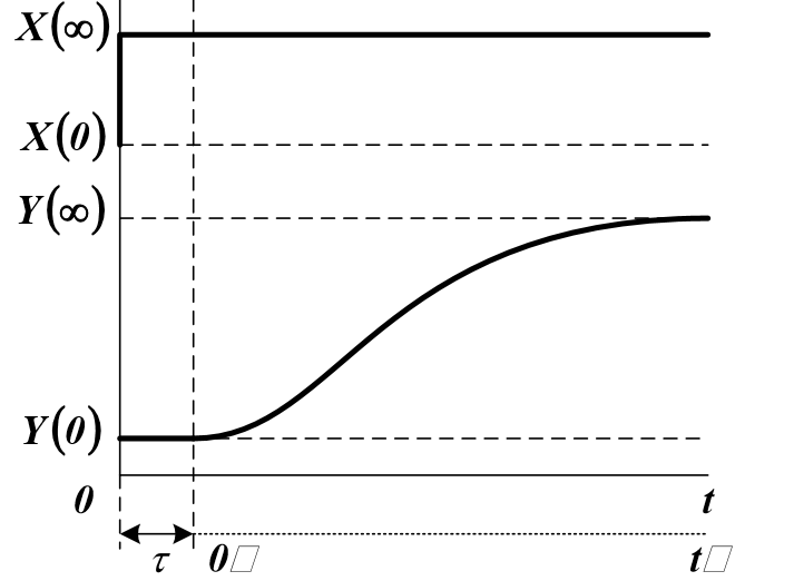
The acceleration curve is the process of the change in time of the output variable, caused by a step input. The acceleration curve is used to determine the dynamic properties of the object.

Formulation of the problem

1. To build mathematical models of dynamic identification of the control object according to the normalized transient response (acceleration curve):

• The method of least squares using derivatives;
• Modified area method.

2. To determine and compare the adequacy of the mathematical models obtained to the control object.

Theory

Identification consists in finding an adequate model for the object. Distinguish between structural and parametric identification. In the case of structural identification, the form of the model is determined from some given class of functions; in parametric identification, the model parameters are determined.

If the output signals of the object Y (t) are completely determined by the observed input effects X (t), then to identify it, it suffices to use the methods of the active experiment.

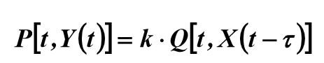
The initial information is the experimentally recorded acceleration curve — the object Y (t) response to the input input action X (t) in the time interval 0≤t≤T.

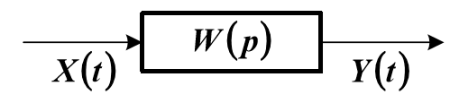
This is a block diagram of an object model with an operator transfer function W (p). The equation of the dynamic characteristics of the object can be represented as follows:

(one)
Where

- lag time of the object, which runs from the moment the signal is given to the input of the object to the moment the signal appears at its output; k - gain (or transfer coefficient) of the object.

Scheme for determining the lag time and the gain of the object:

Input and output values are usually scaled in the standard range from 0 to 1 (normalized):

After determining k and

You can explore the object in normalized coordinates and without delay, by shifting the time scale to the right by

[3].

Structural identification of the object

In structural identification, a priori information about the object is used to determine the structure of the model.

The equation of dynamics, as a rule, is chosen from the class of linear or linearized characteristics. In normalized coordinates, an object model with lumped parameters, one input and one output signal is an ordinary differential equation with constant coefficients:

(2)

where are the coefficients

and

have the dimension of time to a degree equal to the order of the derivative of the corresponding term. In physically realizable systems, n≥m

By the form of the acceleration curve, you can approximately determine the order of a future model, for example, for a first-order object:

For objects of higher orders:

Usually X (t) is a step function, therefore the order of equation (1) can be approximately determined by the shape of the object's acceleration curve. If this characteristic has no inflection points, then n = 1. If there is an inflection at t = t, and t / T <0.1 ... 0.15, then n = 2. Otherwise, consider n> 2. However You can reduce the order of the model by introducing a dummy lag.

Conclusion

The influence of the measurement error X (t) and Y (t) and the error of numerical methods for processing information usually makes it impractical to use models of a higher third or fourth order.

Parametric object identification

With parametric identification, data about an object is processed to obtain a posteriori information about it. The parameters of the selected model are evaluated. In the simplest cases, such an assessment can be performed according to a transient response graph.

Parametric identification by least squares method using derivatives

To identify an object of arbitrary order, the least squares method is used, which requires minimization of the mean square of the residual of the right and left sides of equation (2):

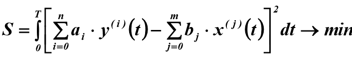(3)

Where:

and

- derivatives of the i-th and j-th order of the functions of the output and input signals.

The solution of problem (3) is reduced to the solution of the system:

(four)

By transforming (4) in accordance with equation (3), one can obtain a system of linear algebraic equations:

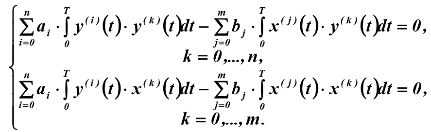(five)

To solve system (5) with respect to unknown parameters

you need to know the derivatives of the input and output signals of the object, which are the result of smoothing the functions X (t) and Y (t) on the segment

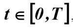. To calculate the coefficient

used formula:

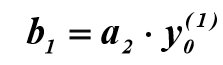
Conclusion

The error of numerical differentiation, as a rule, is quite high, so the scheme for determining the coefficients,

you need to use the differentiation of analytical expressions for X (t) and Y (t).

Parametric identification by the modified area method

To create a model using Python, modifying the area method is on an unchanged time scale. In the classic version, a new time scale is introduced, which, with a numerical solution, leads to an additional error.

Usually, the expression for the transfer function is searched for in one of three mathematical models:

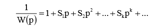
The expression 1 / W (p), the inverse of the transfer function of the model, can be expanded in a series according to degree p:

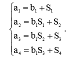
The coefficients a, b of the reduced transfer functions are associated with the coefficients S by the following system of equations:

The coefficients Si are associated with the transition function h (t) by the relations:

(6)

Conclusion

Relations (6) are optimal for solving by means of Python interpolating h (t) with cubic splines, which will be proved by examples.

Assessment of the adequacy of mathematical models of identification of control objects

To select the optimal model, it is sufficient to use the second order adequacy indicator:

(7)

Where

- data taken from the acceleration curve,

- values calculated by the real part Re (W (i × w)) of the transfer function of the model (transition from the frequency domain to the time domain):

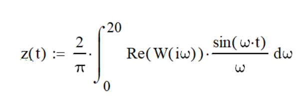(eight)
The best should be considered a model that provides the maximum value.

Considering the significant error of numerical differentiation when solving the system of equations (5), we implement symbolic differentiation. For this, we apply interpolation by a polynomial in accordance with the following listing:

# -*- coding: utf8 -*- import matplotlib.pyplot as plt#    import time start = time.time() import scipy as sp#    import numpy as np#        from sympy import *#     import scipy.integrate as spint from scipy.integrate import quad x=[0.0, 0.4, 0.8, 1.2, 1.6 ,2.0, 2.4, 2.8 ,3.2, 3.6]# y=[0.00, 0.11, 0.36, 0.61, 0.79, 0.89, 0.94, 0.98, 0.99, 1.00]#   fp, residuals, rank, sv, rcond = sp.polyfit(x, y,4, full=True)#   a=round(fp[0],4);b=round(fp[1],4);c=round(fp[2],4) d=round(fp[3],4);e=round(fp[4],4) t=symbols('t ' ,real=True) def h(t):#     h(t) return a*t**4+b*t**3+c*t**2+d*t+e '''   ''' L1=integrate(h(t).diff(t)*h(t).diff(t,t),(t,0,3.6)) L2=integrate(h(t).diff(t,t)*h(t).diff(t,t),(t,0,3.6)) L3=integrate(h(t).diff(t)*h(t).diff(t),(t,0,3.6)) L4=integrate((1-h(t))*h(t).diff(t,t),(t,0,3.6)) L5=integrate((1-h(t))*h(t).diff(t),(t,0,3.6)) """      (5)    (3)""" P= np.zeros([2,2]) P[0,0]=L2;P[0,1]=L1 P[1,0]=L1;P[1,1]=L3 Q= np.zeros([2,1]) Q[0,0]=L4;Q[1,0]=L5 P=np.matrix(P); Q=np.matrix(Q) C=PI*Q '''    ''' a2=C[0,0] a1=C[1,0] b1=C[0,0]*h(t).diff(t).subs(t,0) a2=round(C[0,0],3) a1=round(C[1,0],3) b1=round(C[0,0]*h(t).diff(t).subs(t,0),3) """         (8)""" def ff(x,t): j=(-1)**0.5 return (2/np.pi)*( ((b1*x*j+1)/(a2*(x*j)**2+a1*x*j+1)).real)*(np.sin(x*t)/x) z=np.array([round(quad(lambda x: ff(x,t),0, 20)[0],2) for t in x]) """      (7) """ k=round(1-sum([(y[i]-z[i])**2 for i in np.arange(0,len(y)-1,1)])/sum([(y[i])**2 for i in np.arange(0,len(y)-1,1)]),5) stop = time.time() print ("   :",round(stop-start,3)) plt.title('   \n   -%s'%k) plt.plot(x, y,'o', label='  ') plt.plot(x, z,'r', label=' W=(%s*p+1)/(%s*p**2+%s*p+1)'%(b1,a2,a1)) plt.legend(loc='best') plt.grid(True) plt.show()

We get:

Program working time: 0.802

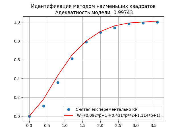
The high degree of adequacy of the model 0.99743 indicates that the resulting transfer function:

W = (0.092 * p + 1) / (0.431 * p ** 2 + 1.114 * p + 1) ,

quite accurately displays the dynamic properties of the object.

The acceleration curve was obtained experimentally; therefore, a further study of object control systems for stability [4] and the determination of controller parameters [5] is of practical importance.

Python implementation of object identification by the modified area method

To solve this problem, you can use numerical methods because the model does not contain differentiation, and the proposed method for solving according to relations (6) does not imply a change in the time coordinate. In addition, we apply spline interpolation in accordance with the following listing:

 # -*- coding: utf8 -*- import matplotlib.pyplot as plt import time start = time.time() from scipy.interpolate import splev, splrep import scipy.integrate as spint import numpy as np from scipy.integrate import quad xx =np.array([0.0, 0.4, 0.8, 1.2, 1.6 ,2.0, 2.4, 2.8 ,3.2, 3.6]) yy =np.array([0.00, 0.11, 0.36, 0.61, 0.79, 0.89, 0.94, 0.98, 0.99, 1.00]) """      """ def h(x): spl = splrep(xx , yy ) return splev(x, spl) """          (6)""" S1=(spint.quad(lambda x:1-h(x),xx[0],xx[len(xx)-1])[0]) S2=(spint.quad(lambda x:(1-h(x))*(S1-x),xx[0],xx[len(xx)-1])[0]) S3=(spint.quad(lambda x:(1-h(x))*(S2-S1*x+(1/2)*x**2),xx[0],xx[len(xx)-1])[0]) S4=(spint.quad(lambda x:(1-h(x))*(S3-S2*x+S1*(1/2)*x**2-(1/6)*x**3),xx[0],xx[len(xx)-1])[0]) """    """ b1=-S4/S3 a1=b1+S1 a2=b1*S1+S2 a3=b1*S2+S3 """    """ def ff(x,t): j=(-1)**0.5 return (2/np.pi)*( ((b1*x*j+1)/(a3*(x*j)**3+a2*(x*j)**2+a1*x*j+1)).real)*(np.sin(x*t)/x) y=np.array([round(quad(lambda x: ff(x,t),0, 20)[0],2) for t in xx]) """     """ k=round(1-sum([(yy[i]-y[i])**2 for i in np.arange(0,len(yy)-1,1)])/sum([(yy[i])**2 for i in np.arange(0,len(yy)-1,1)]),5) stop = time.time() print ("   :",round(stop-start,3)) plt.title('   .\n   -%s'%k) plt.plot(xx, yy,'o', label='   ()') plt.plot(xx, y,'r', label='W=(%s*p+1)/(%s*p**3+%s*p**2+%s*p+1)'%(round(b1,3),round(a3,3),round(a2,3),round(a1,3))) plt.legend(loc='best') plt.grid(True) plt.show()

We get:

Program working time: 0.238

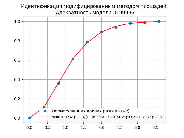
The high degree of adequacy of the model 0.99996 and greater speed than with symbolic differentiation, suggests that the transfer function:

W = (0.074 * p + 1) / (0.067 * p ** 3 + 0.502 * p ** 2 + 1.207 * p + 1)) ,

obtained by the modernized method of areas better displays the dynamic properties of the object.

findings

1. The publication introduces the basics of dynamic identification of the control object.

2. Implementing the solution of the identification problem in the free Python programming language with examples of using the explicit representation of the transition function by a polynomial and splines will help expand the scope of Python.

3. For numerical solutions of identification problems, it is possible to suggest the use of relations (6), which allow one to obtain a result without changing the time coordinate.

Links

Source: https://habr.com/ru/post/345198/

All Articles