Key-value for storing metadata in storage. Testing embedded databases

On November 7-8, 2017, at the Highload ++ conference, researchers at the Radiks Lab presented a report “Cluster Metadata: The Race of Key-Value-Heroes”.

In this article, we presented the main report material relating to testing key-value databases. “Why should they be tested by the storage vendor?” You ask. The task arose in connection with the problem of storing metadata. Such features as deduplication, tearing, thin provisioning (thin provisioning), log-structured recording, run counter to the direct addressing mechanism — there is a need to store a large amount of service information.

Introduction

Suppose that all storage space is divided into pages of size X bytes. Each of them has its own address - LBA (8 Bytes). For each such page we want to store Y bytes of metadata. Thus, we obtain a set of lba -> metadata correspondences. How many such matches will we have? It all depends on how much data we store.
')

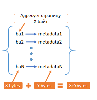
Fig. 1. Metadata

For example, when X = 4KB, Y = 16 bytes. We get the following table:

Table 1. The ratio of storage volume and metadata

The amount of data per node	Number of keys per node	Metadata volume
512TB	137 billion	3TB
64TB	17 billion	384GB
4TB	1 billion	22.3GB

The volume of metadata is quite large, so keeping metadata in RAM is not possible (or it is not economically feasible). In this regard, the question arises of storing metadata, and with maximum access performance.

Metadata storage options

1. Key-value DB. lba - key, metadata - value
2. Direct Addressing. Do not store lba = N * Y metadata, not N * (8 + Y) B

What is direct addressing? This is when we simply place our metadata on the drive in order, starting with the very first sector of the drive. At the same time, we don’t even have to write down to which lba the metadata correspond, since everything is in ascending order of lba.


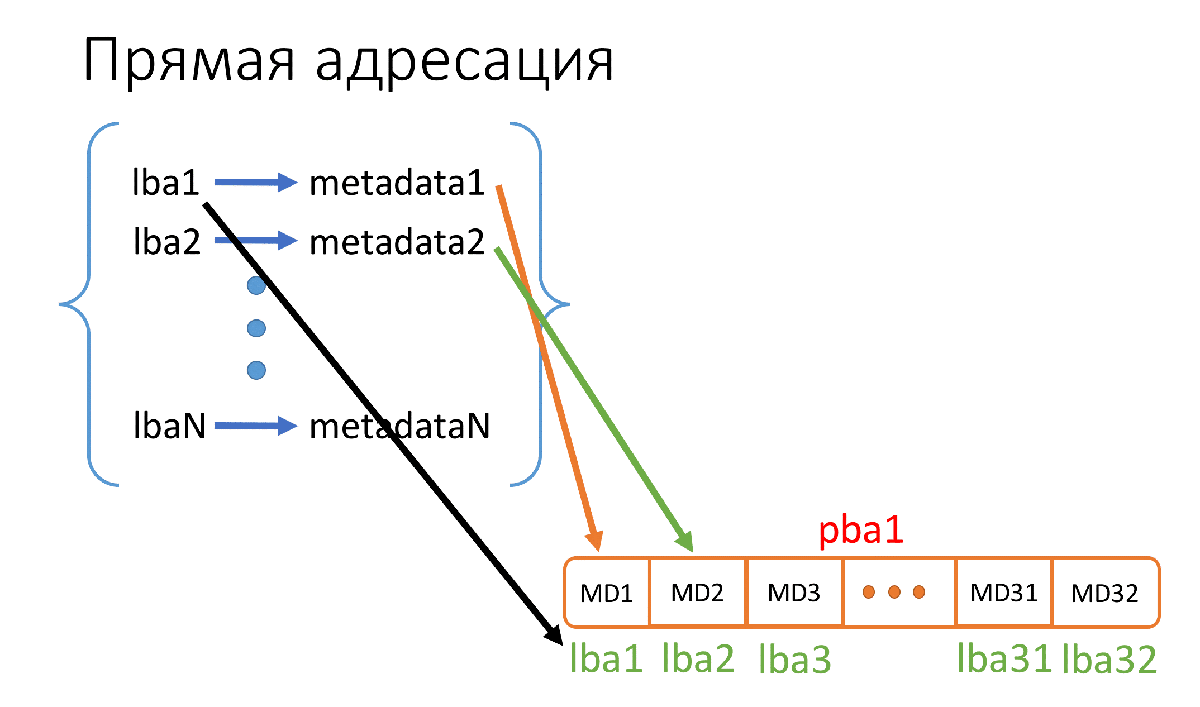
Fig. 2. The principle of direct addressing

In Figure 2, pba1 is the physical sector (512B) of the drive, where we store metadata, and lba1 ... lba32 (there are 32 of them, because 512 / 16 = 32) are the addresses of the pages with which this metadata corresponds, and these we do not need to store addresses.

Analysis of the workload in the storage system

Based on our experience of workloads, we decide what requirements for delays and throughput we need.

Workload in the media industry :

• NLE (non-linear editing) - reading and writing several large files in parallel.
• VOD (video on demand) - reading multiple streams, sometimes with jumps. It is possible to write in parallel in several streams.
• Transcoding - 16–128 KB random R / W 50/50.

Enterprise workload:

• 8–64 KB IO.
• Random read / write approximately 50/50.
• Periodically Seq Read and Write to hundreds of threads (Boot, Virus Scan).

Workload in high performance computing (HPC) :

• 16/32 KB IO.
• Alternate read / write in hundreds and thousands of threads.

From the presented workloads in various sectors of the market we will form the final performance requirements for All-Flash DSS:

1. Show:
   • Latency (latency) 1–2ms (99.99% percentile) for flash.
   • From 20GB / s, from 300–500k IOPS.
2. On the following loads:
   • Random R / W.
   • Ratio 50/50.
   • Block size 8–64K.

To choose which database of the dozens of existing ones will suit us, it is necessary to conduct tests on selected loads. So we can understand how a database deals with a certain amount of data, which provides latency / throughput.

What difficulties arise at the start?

1. We'll have to select only a few databases for tests - everything will fail to test. How to choose these few? Only subjectively.
2. Ideally, you should carefully configure each database before testing, which can take an enormous amount of time. Therefore, we decided to first look at what numbers can be obtained in the standard configuration, and then decide how promising the testing is.
3. It is rather difficult to make tests completely objective and create the same conditions for each of the databases due to fundamental differences between the databases.
4. Few benchmarks or difficult to find. What we need is unified benchmarks that can be used to test any (or almost any) key-value database, or at least some of the most interesting ones. When testing different databases with different benchmarks, objectivity suffers.

Types of key-value database

There are two types of key-value databases:

1. Embedded - they are also called "engines". In fact, this is a library that you can connect to in your code and use its functions.
2. Dedicated - you can also call them “database server”, “NoSQL database”. These are separate processes that can most often be accessed by sockets. Usually have more features than embedded. For example, replication.

In this article we will consider testing embedded key-value databases (hereinafter, we will call them "engines").

What to test?

The first option that can be found is YCSB .

Features YCSB:

• This benchmark is a kind of industry standard, they trust it.
• Workloads can be easily configured in configuration files.
• Written in Java. In this case, it is a minus, because Java is not very fast, and this can introduce distortion into the test results. In addition, the engines are mainly written in C / C ++. This makes it difficult to write the driver YCSB <-> engine.

The second option is a benchmark for ioarena engines.

• Written in C.
• Few workloads. Of those that interest us, there is only Random Read. We had to write in the code we need workloads.

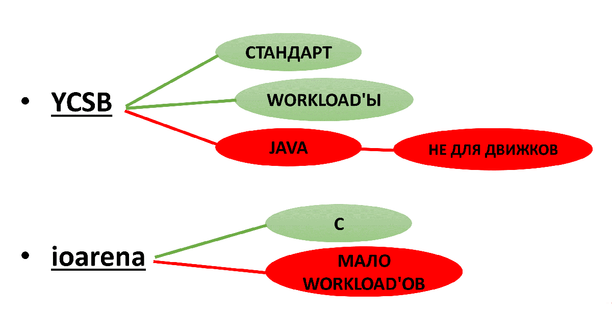
Fig. 3. Testing options

As a result, ioarena is selected for the engines, and YCSB is selected for the selected ones.

In addition to the workloads in ioarena, we added an option (-a), which allows you to specify the number of operations performed per thread and the number of keys in the database separately when running.

All changes to the ioarena code can be found on GitHub .

Test parameters of the key-value database

The main workload that we are interested in is Mix50 / 50. We also decided to look at RR, Mix70 / 30 and Mix30 / 70 in order to understand which databases more “love” this or that workload.

Testing method

We test in 3 stages:

1. Database filling - we fill in 1 database flow to the required number of keys.
   1.1 Reset caches! Otherwise, the tests will be dishonest: the database usually writes data on top of the file system, so the operating system cache works. It is important to discard it before each test.
2. Tests for 32 threads - we run workloads
   2.1 Random Read
   • We reset caches!
   2.2 Mix70 / 30
   • We reset caches!
   2.3 Mix50 / 50
   • We reset caches!
   2.4 Mix30 / 70
   • We reset caches!
3. Tests for 256 threads.
   3.1 Same as for 32 threads.

What are we measuring?

• Throughput / throughput (IOPS / RPS - who loves which notation).
• Latency (msec) latency:
  • Min.
  • Max.
  • The mean square value is a more significant value than the arithmetic mean, because takes into account the standard deviation.
  • Percentile 99.99.

Test environment

Configuration:

CPU:	2x Intel Xeon E5-2620 v4 2.10GHz
RAM:	16GB
Disk:	[2x] NVMe HGST SN100 1.5TB
OS:	CentOS Linux 7.2 kernel 3.11
FS:	EXT4

It is important to note here that such a small amount of RAM is taken not by chance. Thus, the base will not be able to fit completely into the cache on tests with 1 billion keys.

The amount of available RAM was not physically regulated, but programmatically - part of it was artificially filled with a Python script, and the remainder was free for the database and caches.

In some tests there was a different amount of available memory - this will be discussed separately.

NVMe in tests used one.

Write reliability

An important point is the reliability mode of writing data to disk. From this very much depends on the recording speed and the probability / volume of losses in case of failures.

In general, there are 3 modes:

• Sync - fair write to disk before answering the “OK” user for a write request. In the event of a failure, everything remains in place until the last committed transaction.
• Lazy - we write data to the buffer, we answer the user with “OK”, and after a short period of time we buffer the buffer to disk. In case of failure, we may lose some recent changes.
• Nosync - we don’t flush data to disk and just write them to the buffer so that sometime (not fundamentally when) to flush the buffer to disk. In this mode there can be big losses in case of failure.

By performance, the difference is approximately the same (for example, MDBX engine):

• Sync = 10k IOPS
• Lazy = 40k IOPS
• Nosync = 300k IOPS

The numbers here are ONLY for an approximate understanding of the difference between modes.

As a result, for tests, the lazy mode was chosen as the most balanced. Exceptions will be discussed separately.

We test the embedded key-value database

To test the “engines” we performed two test options: for 1 billion keys and for 17 billion keys.

Selected "engines":

• RocksDB - everyone knows about it, this is a database from Facebook. LSM index.
• WiredTiger - MongoDB engine. LSM index. Read here .
• Sophia - this engine has its own custom index, which has something in common with LSM-trees, B-trees. You can read here .
• MDBX - fork LMDB with improvements in reliability and performance. B + tree as an index.

Test results. 1 billion keys

Filling

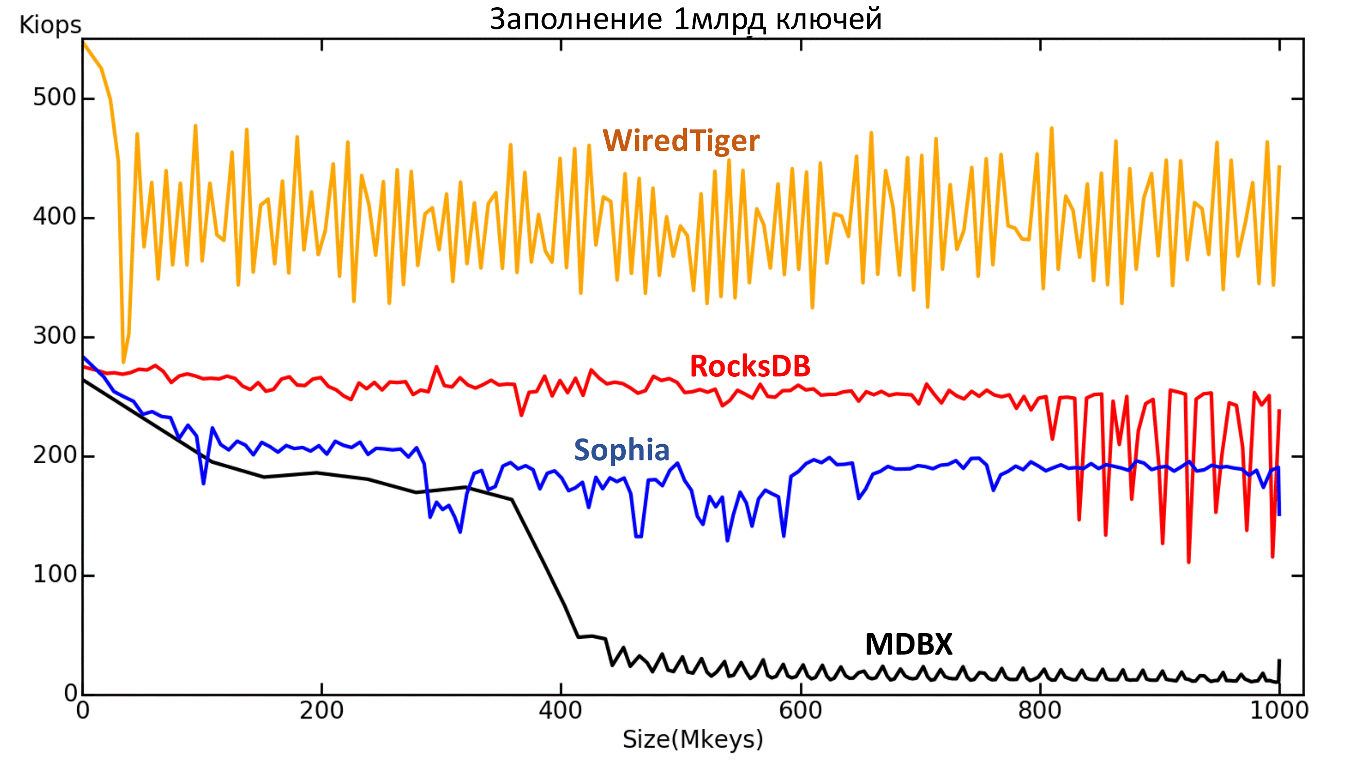
Fig. 4.1. Dependence of the current speed (IOPS) on the number of keys (the x-axis - millions of keys).

Here are all the engines in the standard configuration. Reliability mode Lazy, except MDBX. His record is too slow in Lazy, so the Nosync mode was chosen for him, otherwise the filling will take too long. However, it is clear that from some point the recording speed still drops to about the speed level of the Sync mode.

What can be seen on this chart?

First , something happens to RocksDB after 800 million keys. Unfortunately, the reasons for what is happening have not been clarified.


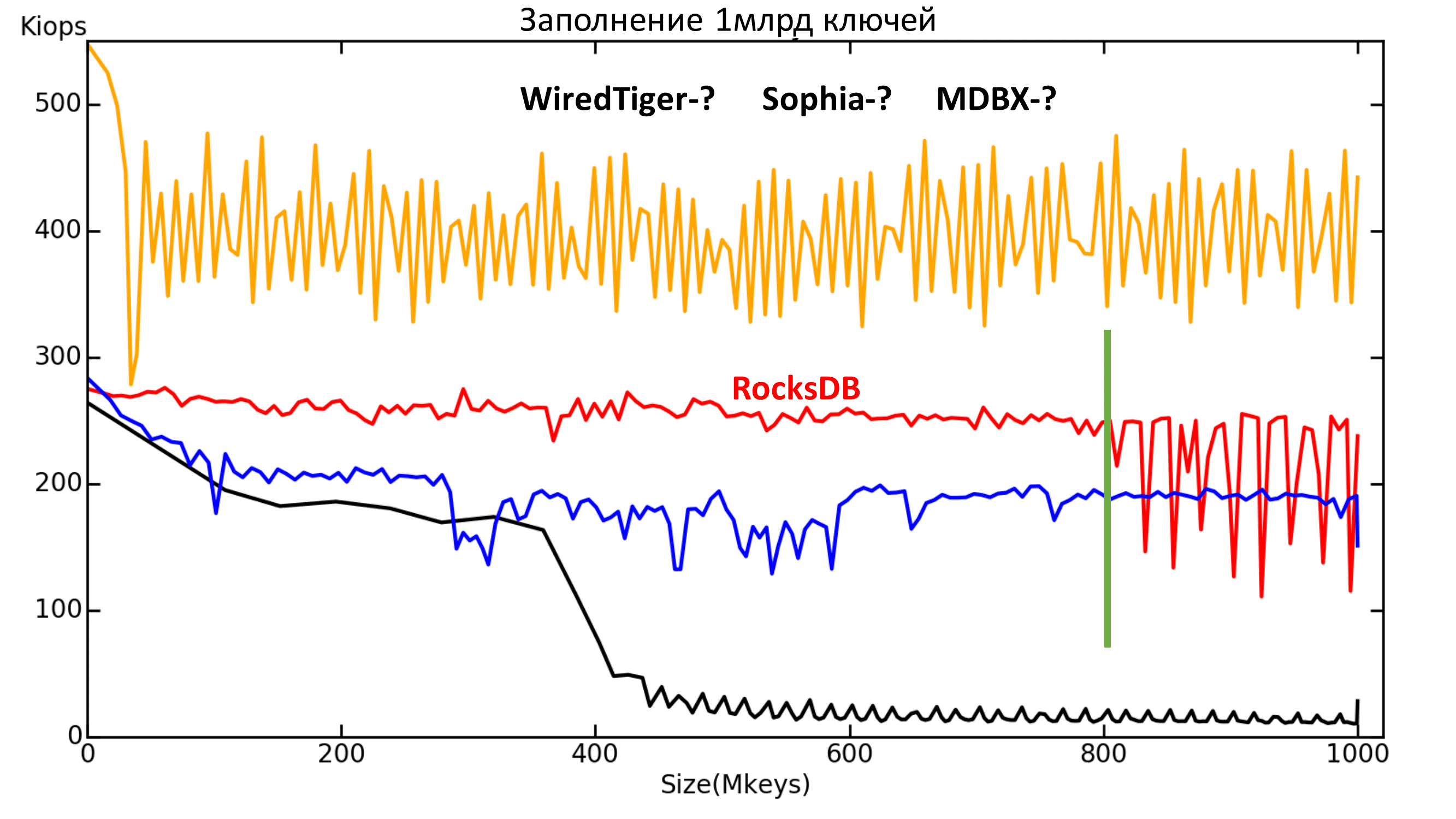
Fig. 4.2. Dependence of the current speed (IOPS) on the number of keys (the x-axis - millions of keys).

Second: MDBX didn’t tolerate the moment when data became more than the available memory.


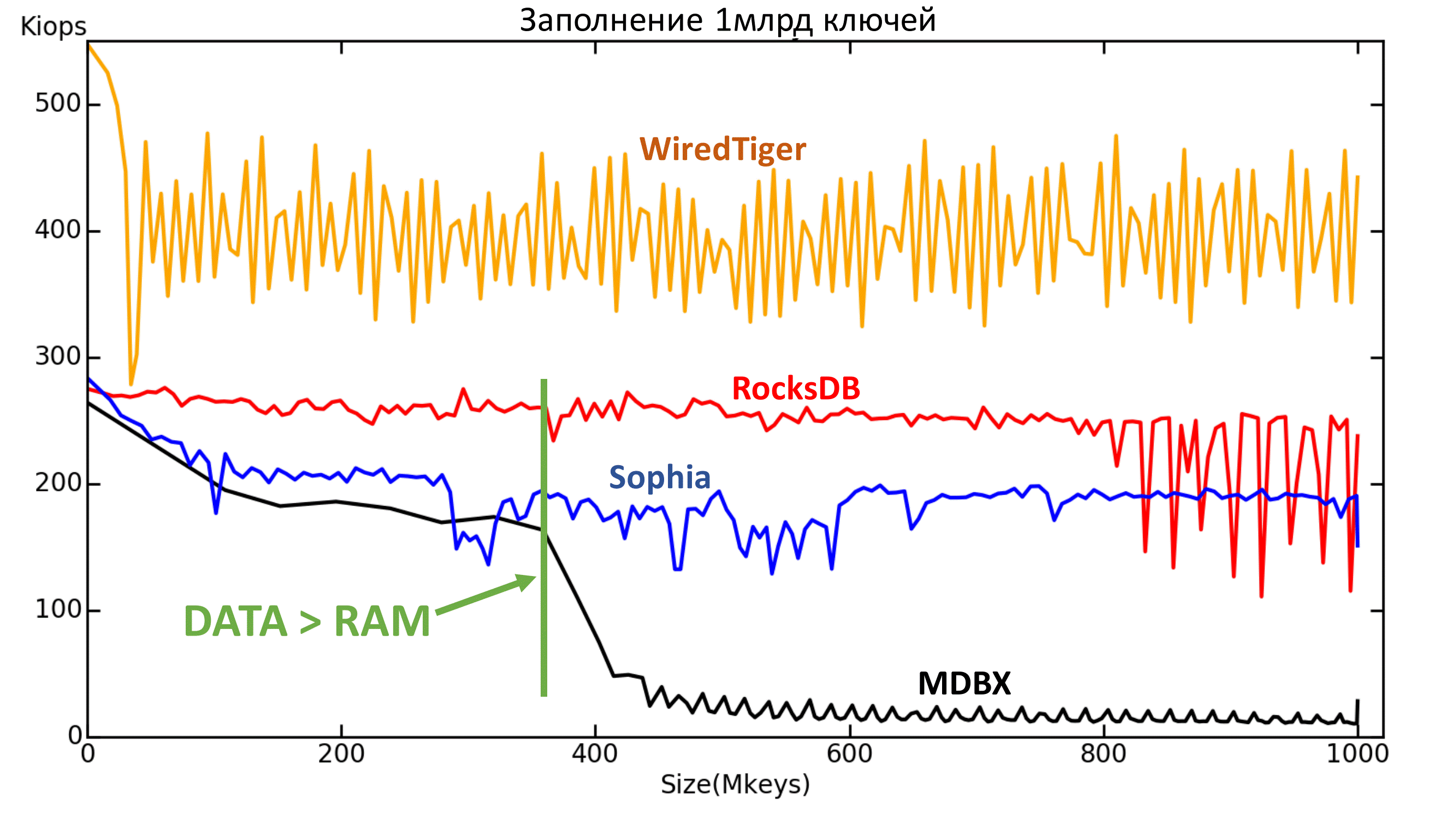
Fig. 4.3. Dependence of the current speed (IOPS) on the number of keys (the x-axis - millions of keys).

Then you can look at the maximum delay graph. It also shows that RocksDB started flights after 800 million keys.


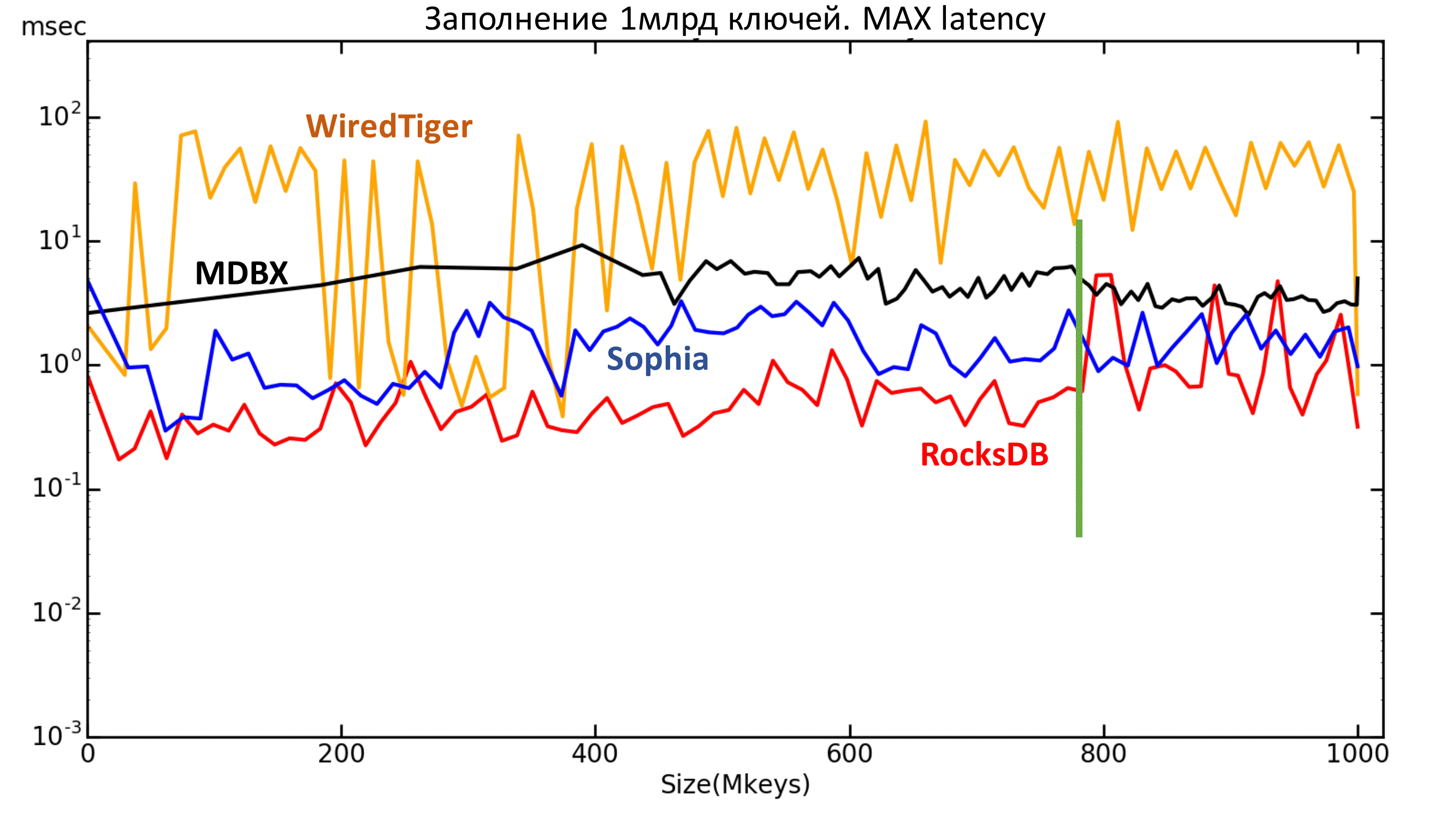
Fig. 5 Maximum latency

Below is a graph of the average quadratic delay value. You can also see the very same borders for RocksDB and MDBX.


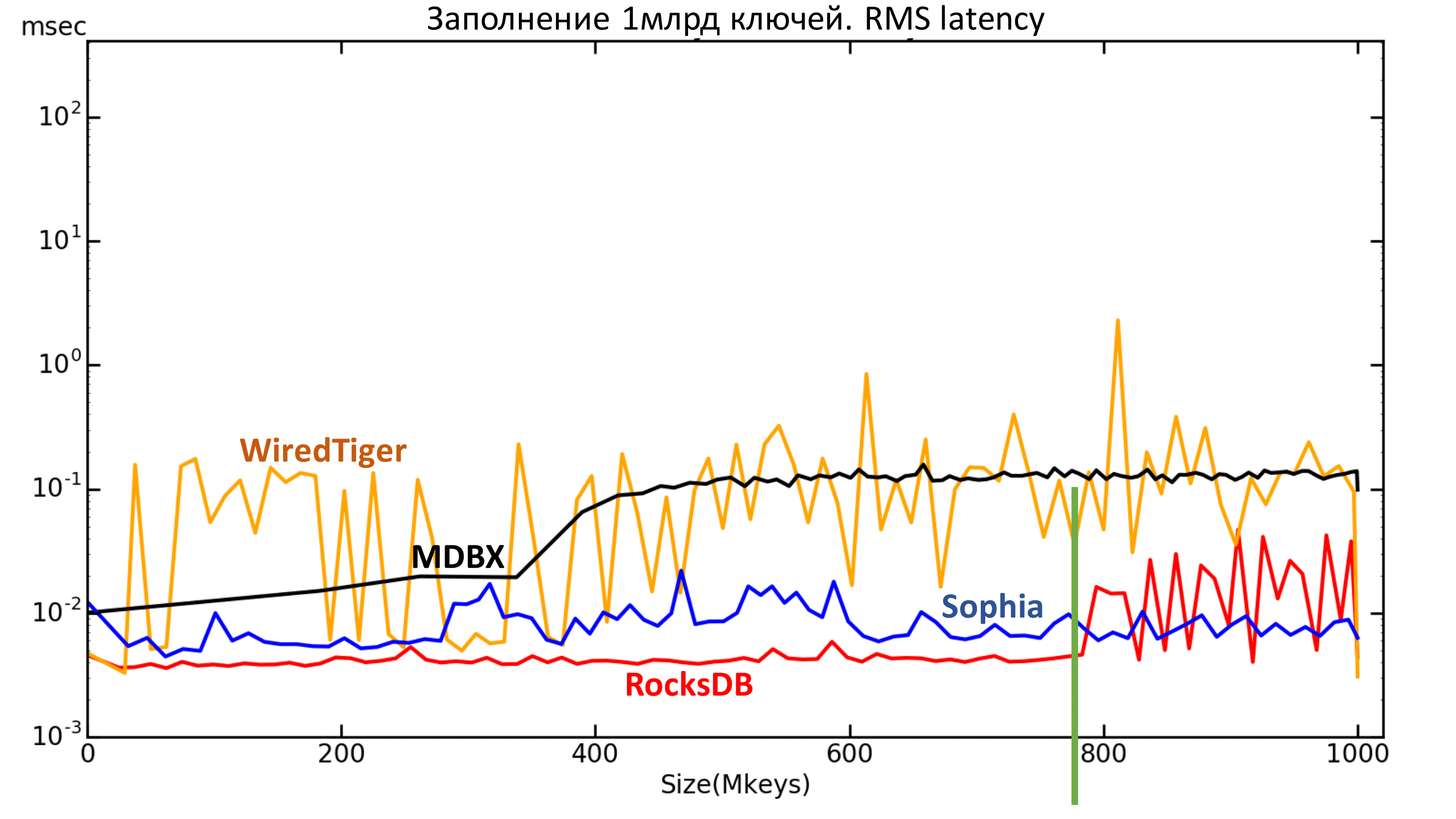
Fig. 6.1. RMS Latency


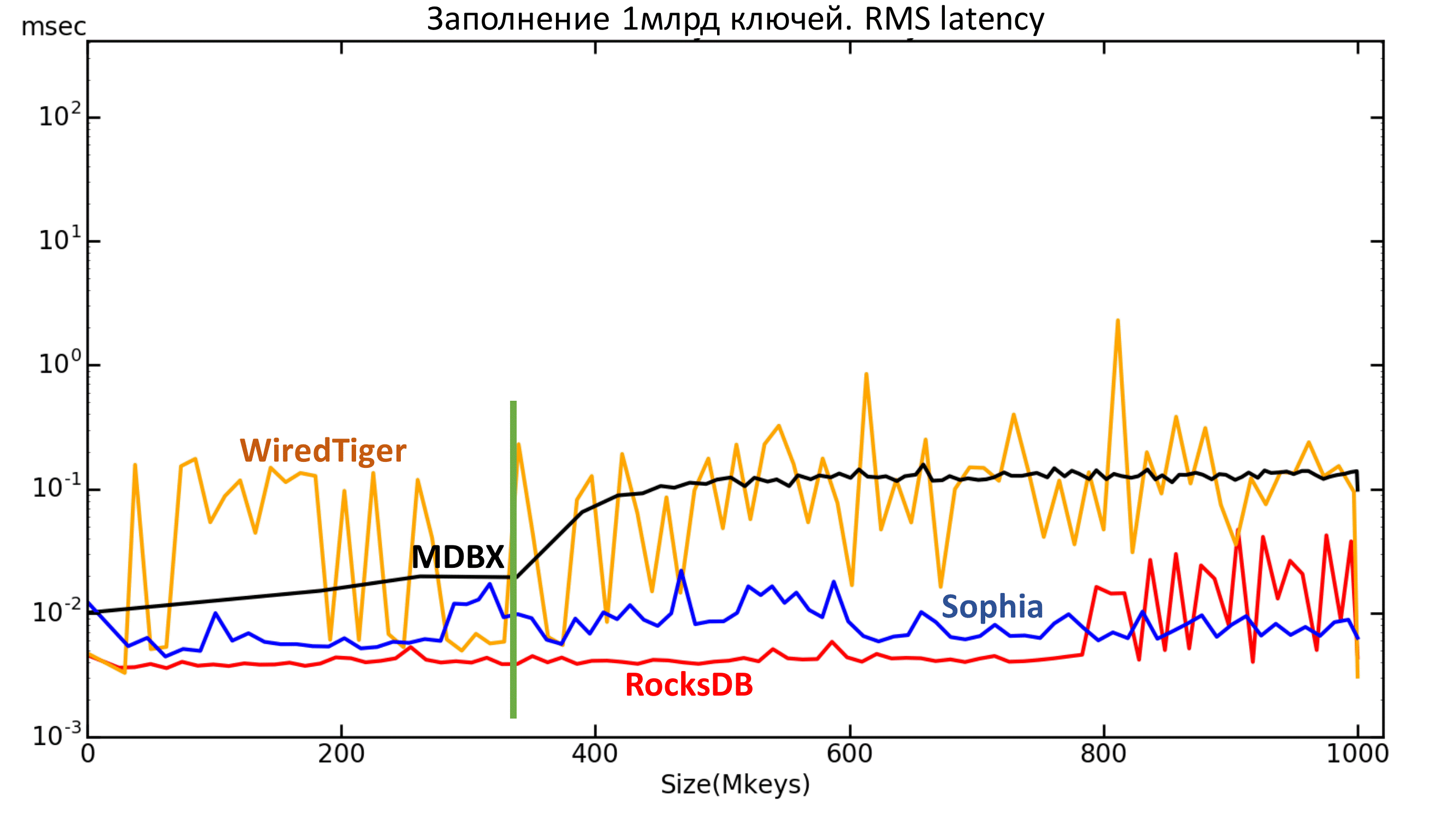
Fig. 6.2. RMS Latency

Tests

Unfortunately, Sophia showed low results in all tests. Most likely, she does not “love” many streams (ie, 32 or more).

WiredTiger first showed very poor performance - at the level of 30 IOPS. It turned out that he has an important parameter cache_size, which by default is set to 500MB. After installing it on 8GB (or even 4GB), everything becomes much better.

For the sake of interest, a test was conducted with the same amount of data, but with the amount of available memory> 100GB. In this case, MDBX with a margin goes forward in the reading test.


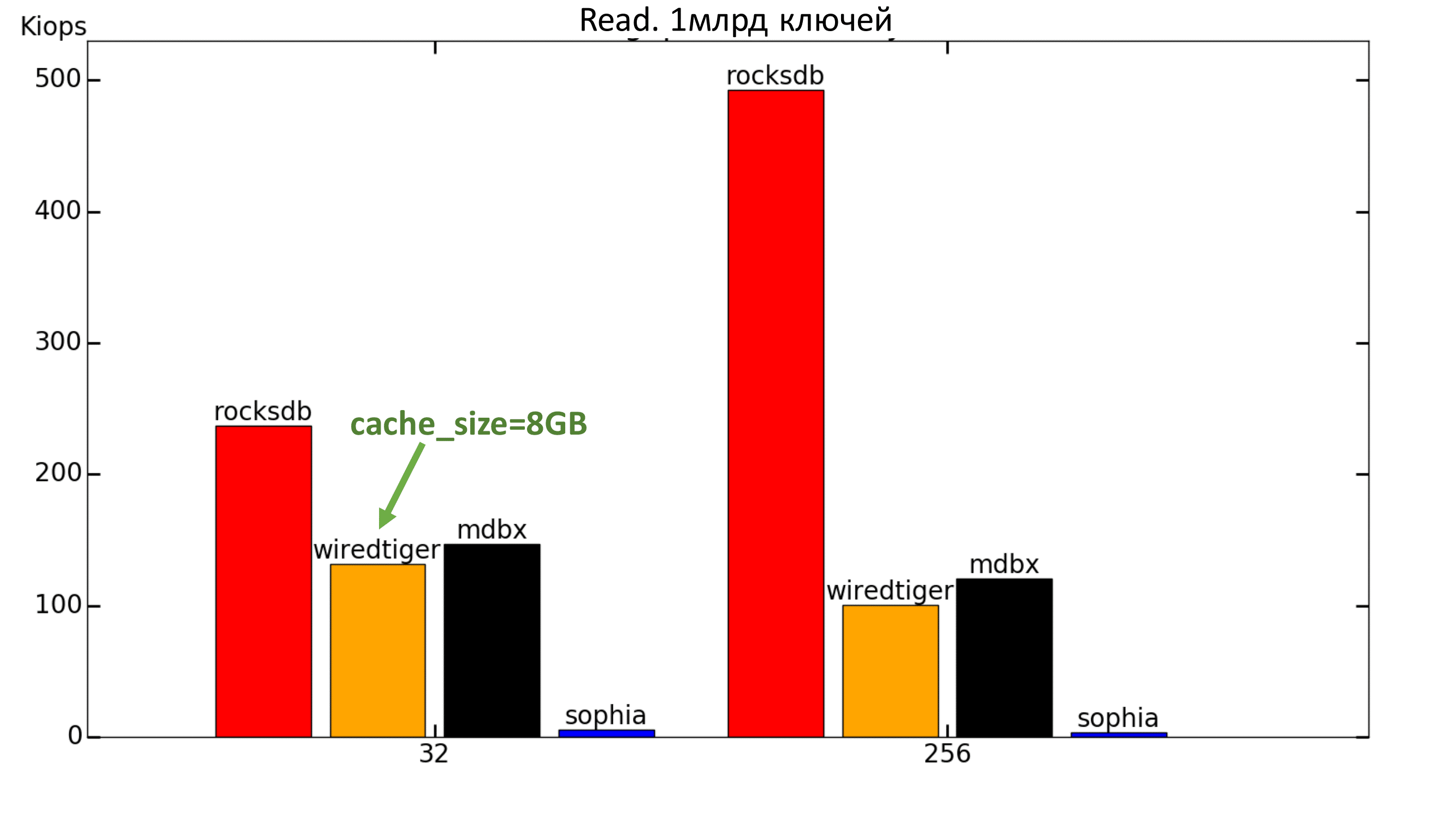
Fig. 7. 100% Read

When adding a record to workload, we get a strong drop in MDBX (which is expected, because the speed was low when filling). WiredTiger grew, and RocksDB slowed down.


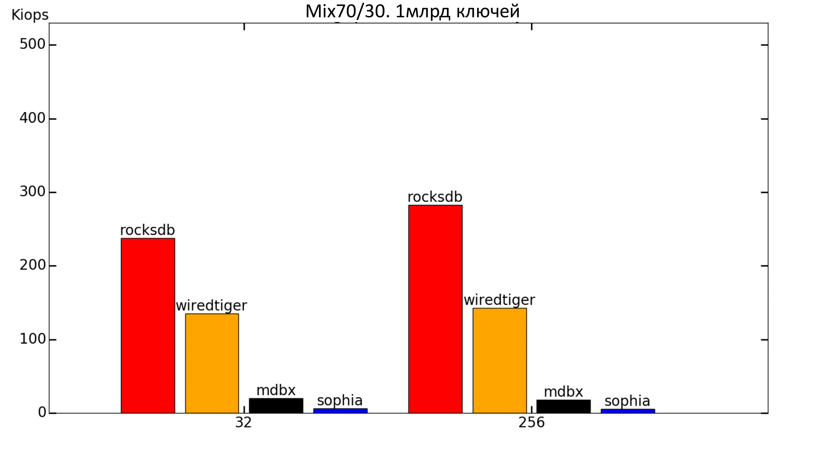
Fig. 8. Mix 70% / 30%

The trend is preserved.


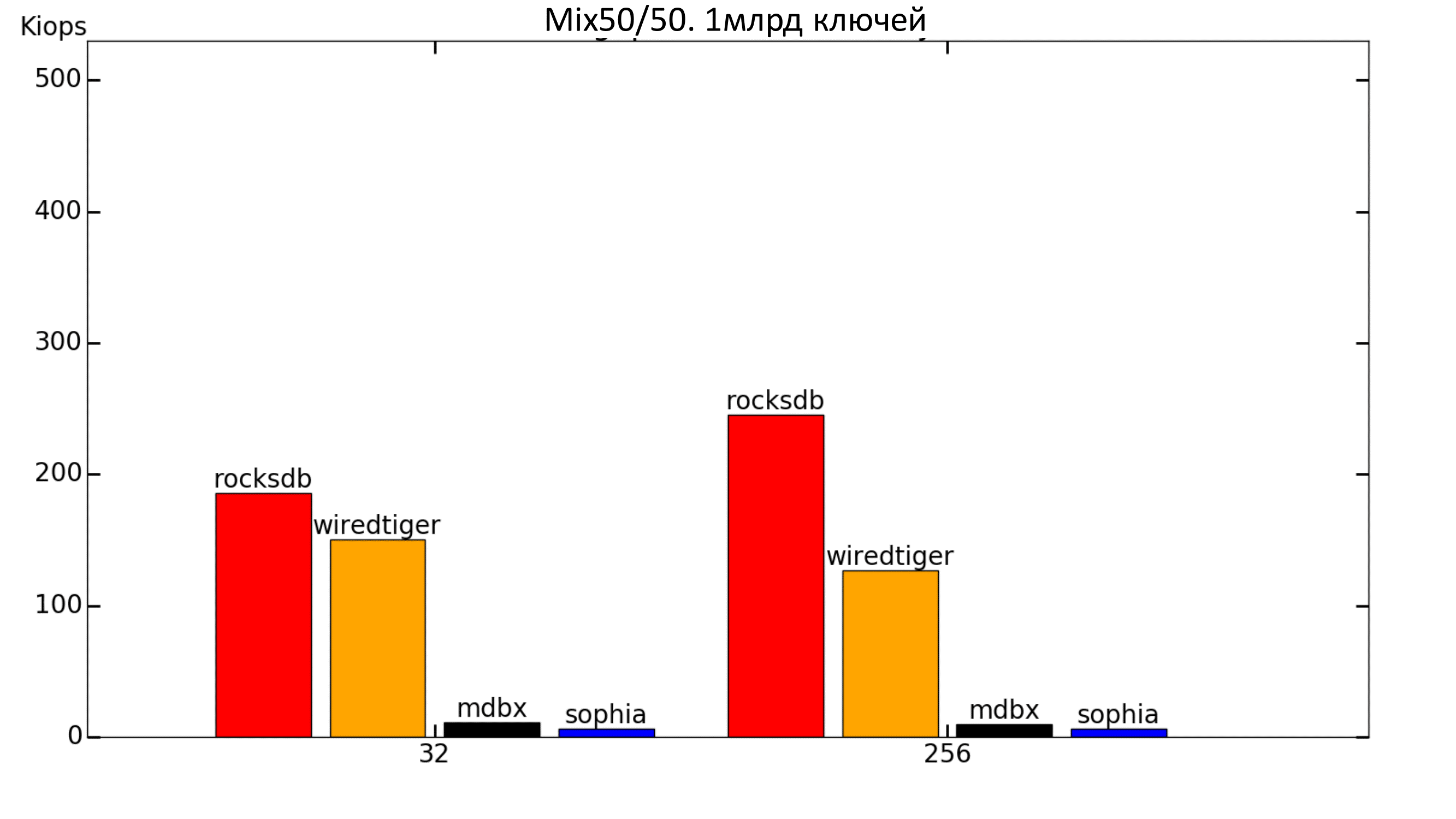
Fig. 9. Mix 50% / 50%

When there are a lot of recordings, WiredTiger begins to overtake RocksDB on a small number of threads.


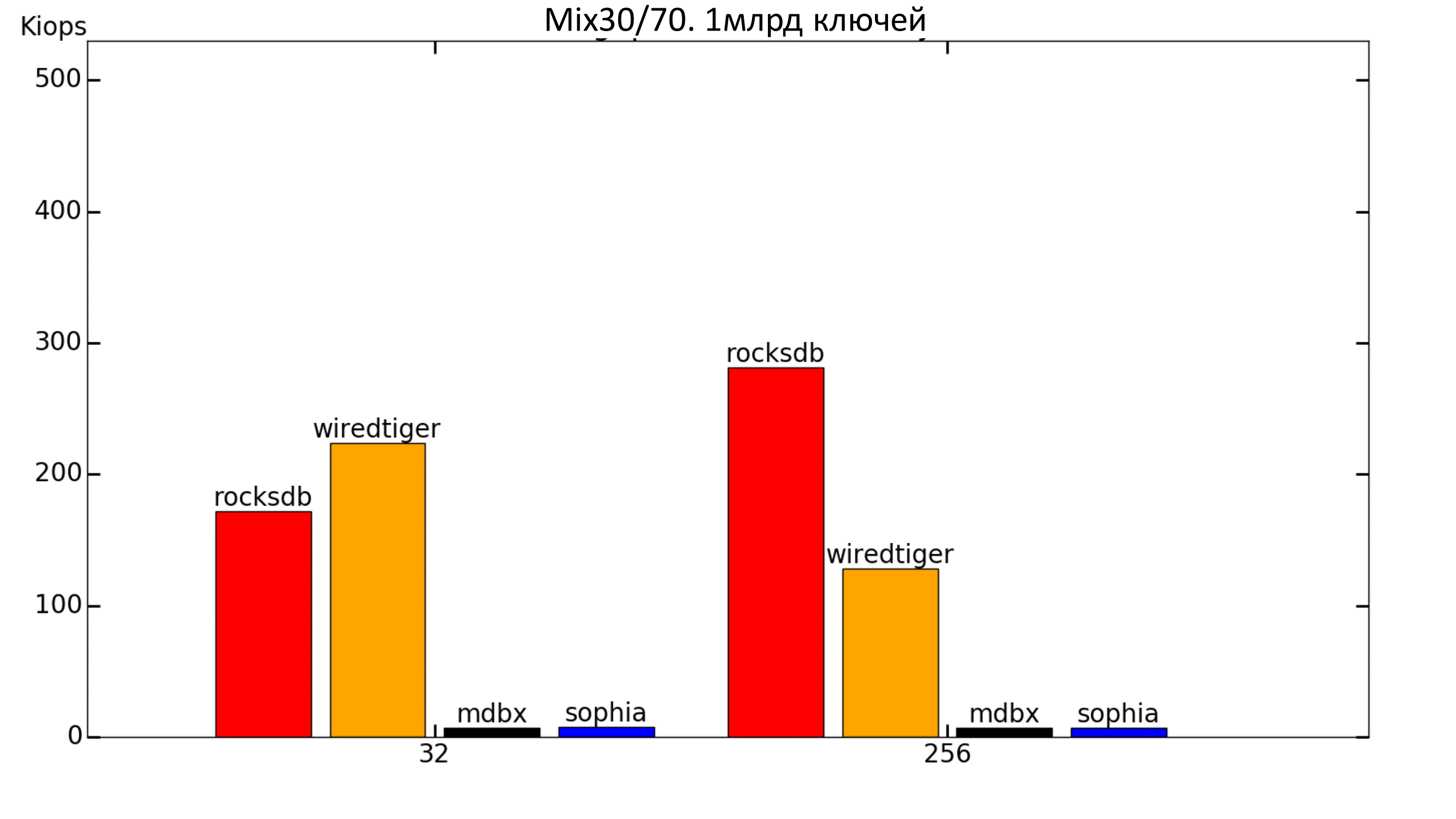
Fig. 10. Mix 30% / 70%

Now you can look at the graphics delays. The columns show the minimum and maximum delays, the orange bar shows the average quadratic delay, and the red bar shows the percentile 99.99.

The green bar is about 2 ms. That is, we want the percentile to be no higher than the green bar. In this case, we do not get this (logarithmic scale).


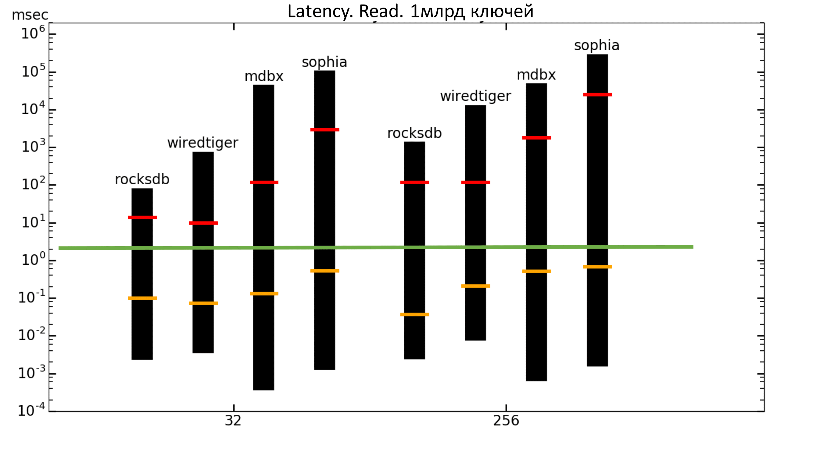
Fig. 11. Latency Read


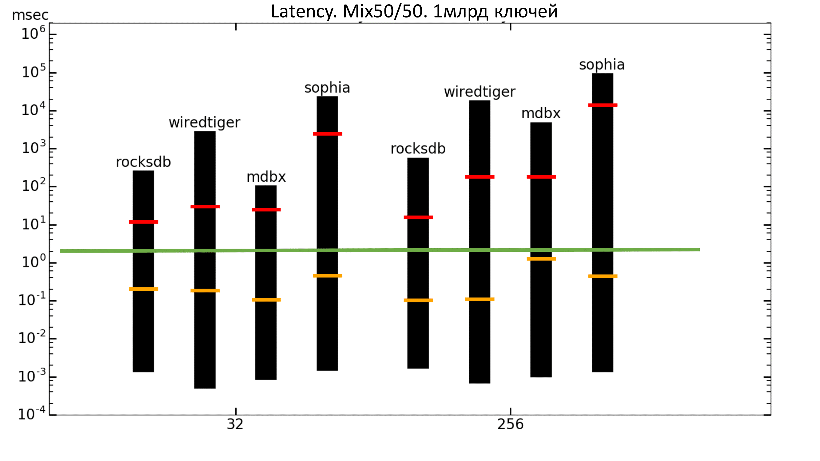
Fig. 12. Latency 50% / 50%

Test results. 17 billion keys

Filling

Tests for 17 billion keys were conducted only on RocksDB and WiredTiger, because they were the leaders in tests for 1 billion keys.

WiredTiger started having strange attacks, but in general it shows itself quite well on filling, plus there is no degradation with increasing data.

But RocksDB eventually went below 100k IOPS. Thus, in the test for 1 billion keys, we did not see the whole picture, so it is important to conduct tests on volumes comparable to real ones!


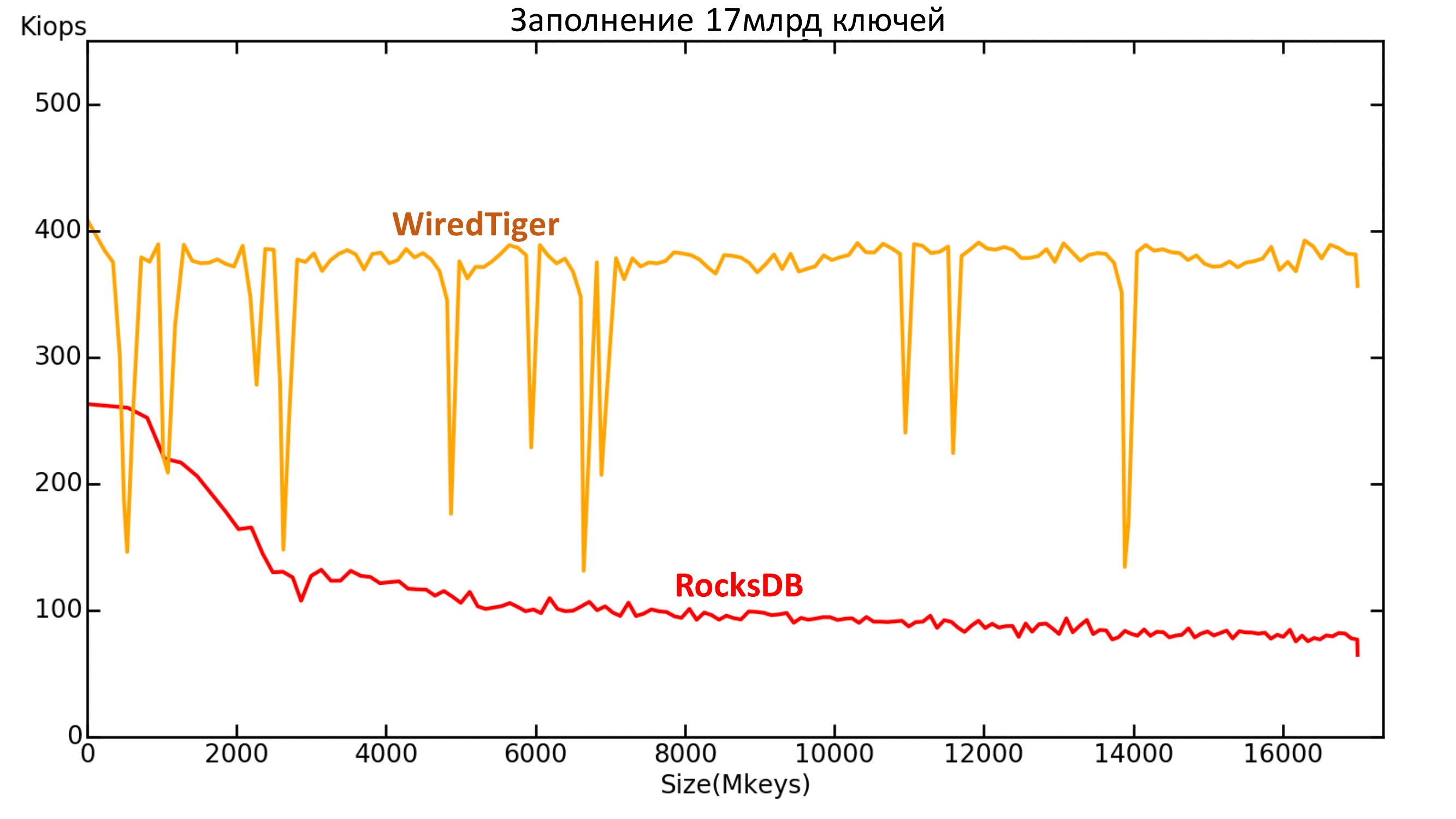
Fig. 13. Productivity 17 billion keys

The dotted line shows the mean square delay. It can be seen that the maximum delay for WiredTiger is higher, and the average quadratic delay is lower than that of RocksDB.


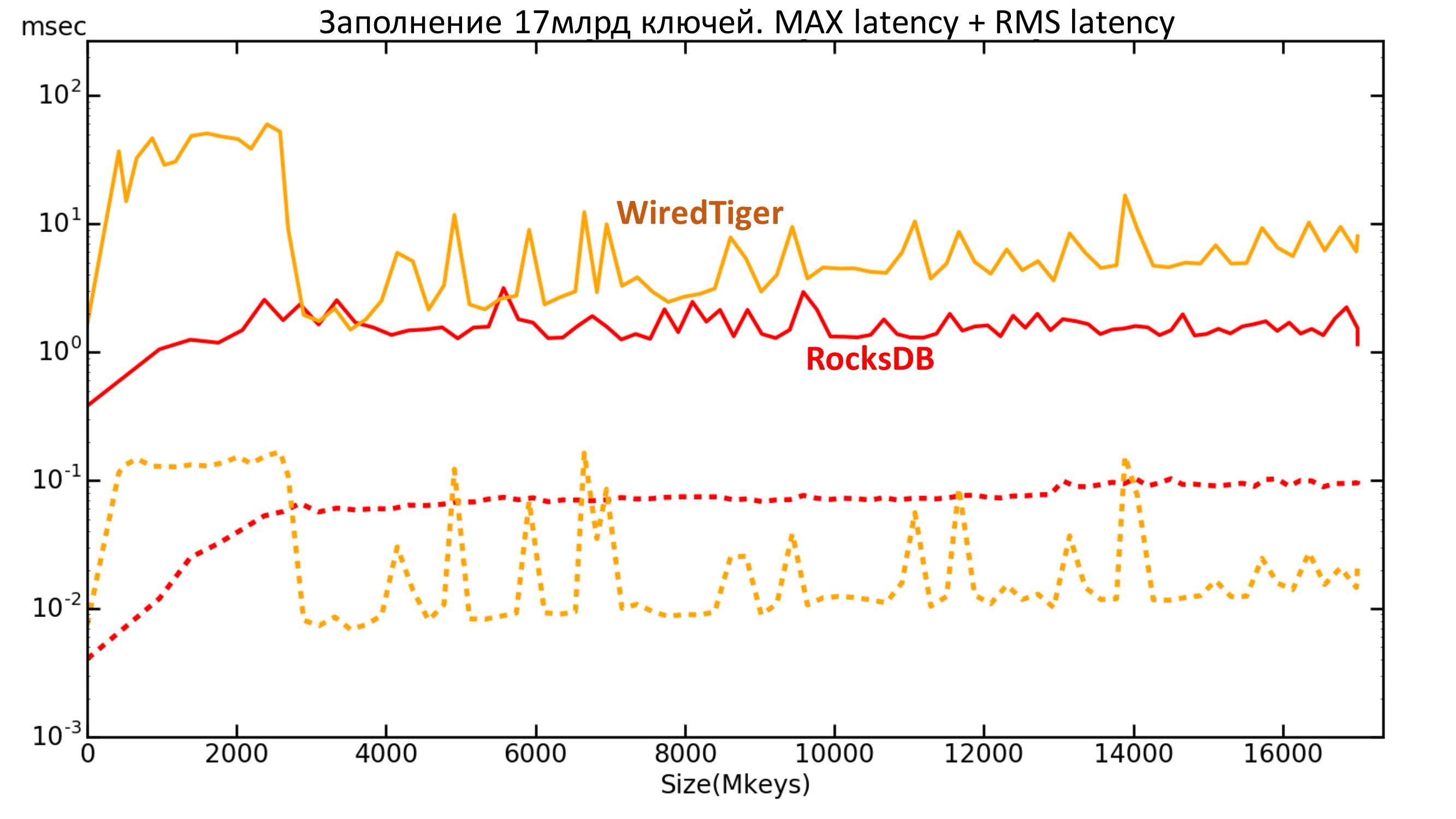
Fig. 14. Latency 17 billion keys

Tests

WiredTiger had the same trouble as last time - it showed about 30 IOPS per read, even with cache_size = 8GB. It was decided to further increase the value of the cache_size parameter, but this did not help either: even with 96GB, the speed did not rise above several thousand IOPS, although the allocated memory was not even full.

When adding a record to the workload, WiredTiger traditionally rises.


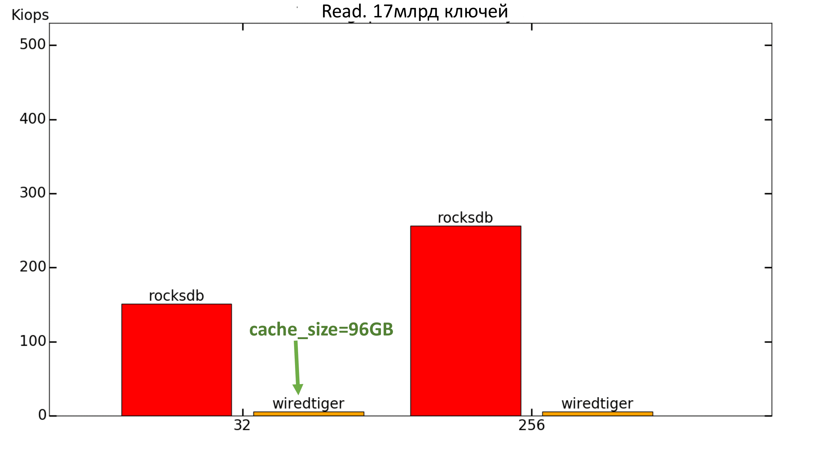
Fig. 15. Performance 100% Read


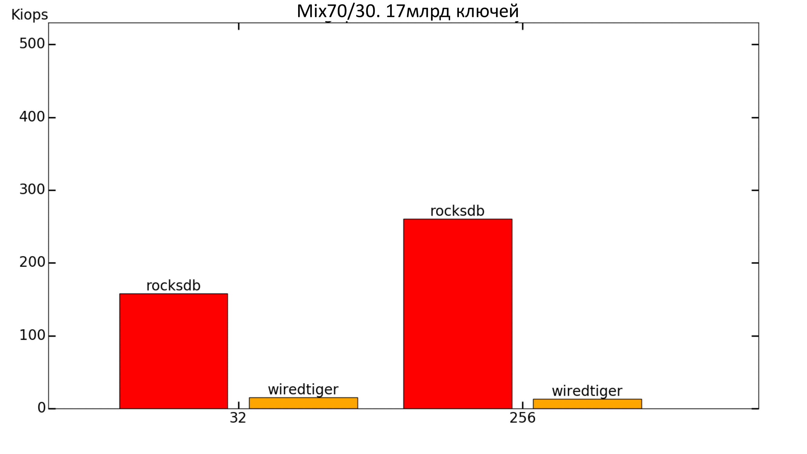
Fig. 16. Productivity 70% / 30%


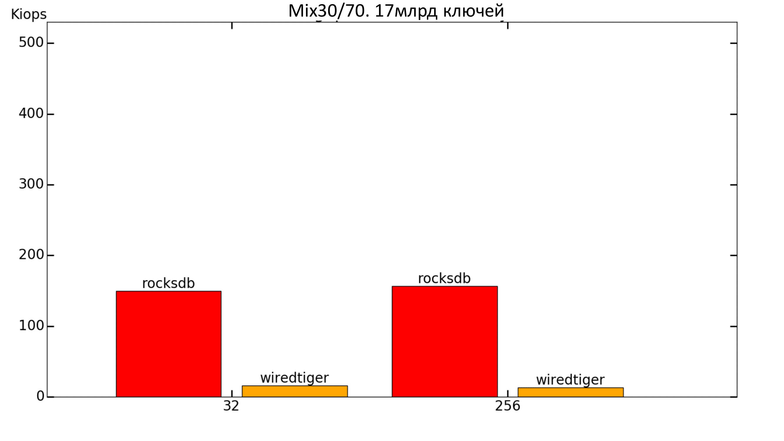
Fig. 17. Productivity 30% / 70%


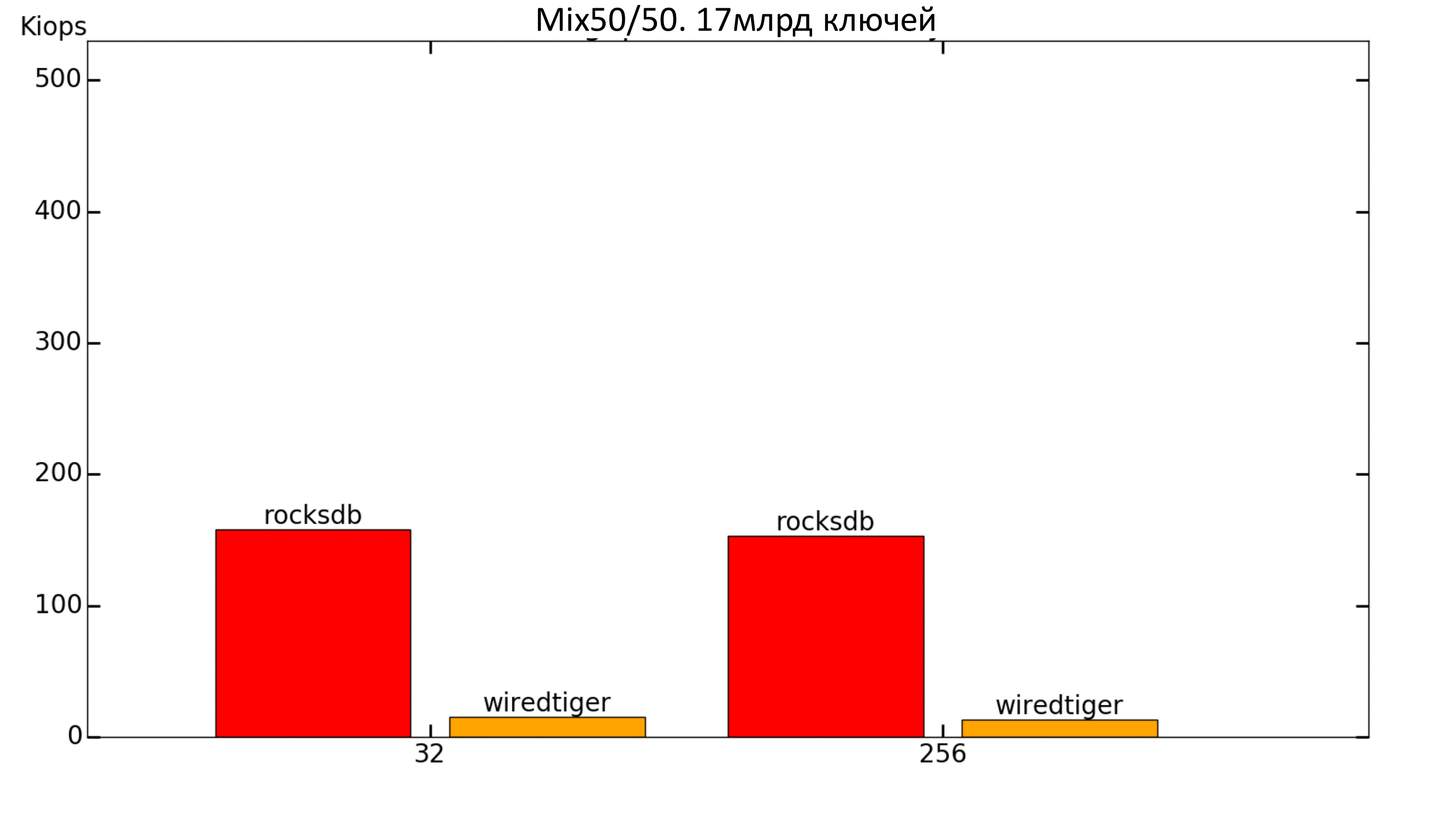
Fig. 18. Productivity 50% / 50%


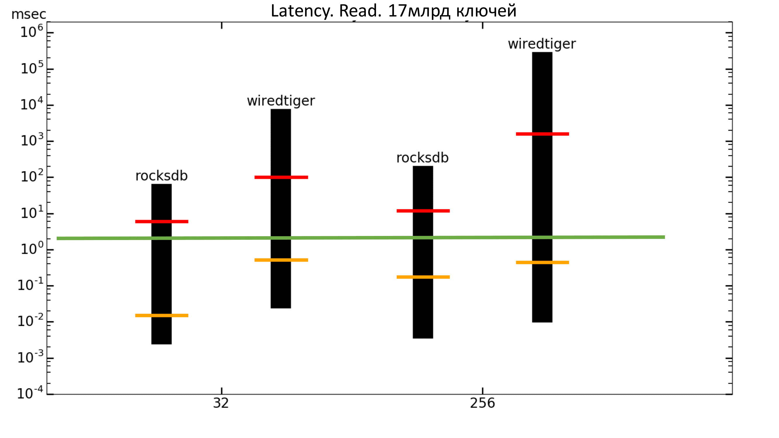
Fig. 19. Latency 100% Read


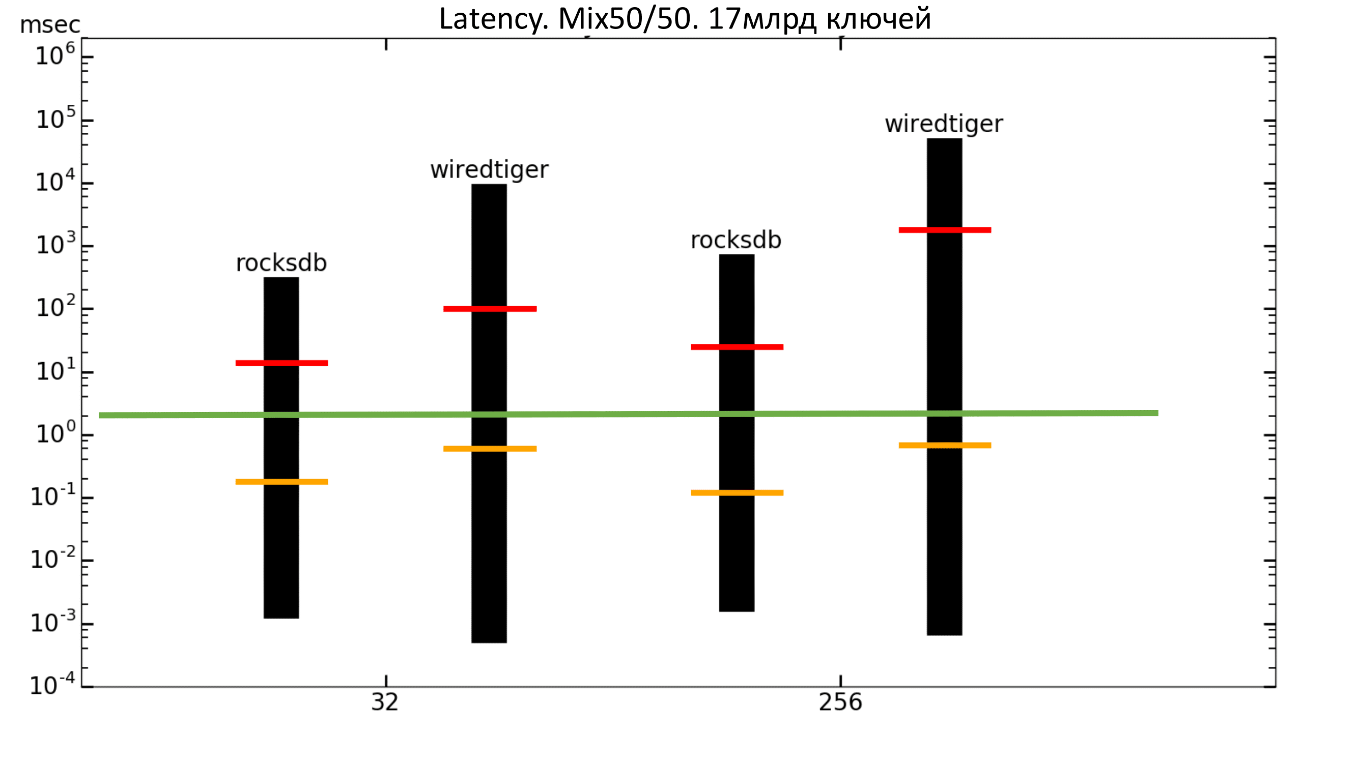
Fig. 20. Latency 50% / 50%

findings

From what has been said above, we can draw the following conclusions:

For a base of 1 billion keys:

• Record + few threads => WiredTiger
• Record + many threads => RocksDB
• Read + DATA> RAM => RocksDB
• Read + DATA <RAM => MDBX

From which it follows that:

• Mix50 / 50 + many threads + DATA> RAM => RocksDB

For a base of 17 billion keys: a clear lead from RocksDB .

This is the situation with embedded engines. In the next article we will talk about the indicators of the selected key-value databases and draw conclusions about benchmarks.