Evaluation of option premiums - analytical formulas vs modeling

Introduction

In the wake of HYIP cryptocurrency slips news about Bitcoin trading on the CME and NASDAQ world exchanges. For me, this is a landmark event: the hands of corporations that inflated dot-com and mortgage bubbles reached out to the gold of the crypank, cryptocurrency. And in the arsenal of these same corporations a powerful lever - derivative financial instruments, or derivatives.

Being impressed by the history of the ups and metamorphosis of the derivatives markets that I read not so long ago — above all, futures and option contracts, I became interested in the non-trivial pricing of options. I discovered that although the Internet is full of rewrites of articles interpreting the famous Black-Scholes formula, practical tools — web sites, technology programs, or banal programmer’s guides — are not mathematics, this issue is lacking on the Internet. I had to remember the basics of the server and adapt rigorous mathematical descriptions in a popular, understandable, first of all, to me, format.

Option Definition

An option is a contract that gives the buyer the right (but not the obligation!) To buy or sell an asset that is traded on the market at the price indicated by him (the contract buyer). The option seller assigns a premium to the buyer - his remuneration for the opportunity given to the option buyer to buy or sell an asset in a certain period at a certain price.
Example of an option contract:

• option buyer wants to get the right to buy 10 Ethereum (ETH) at a price of $ 470 for 1 ETH in 30 days.
• Ethereum's current price is $ 450.

Suppose that in 30 days the market rate of Ethereum will rise to $ 500. The buyer of the option will be able to buy 10 Ethereum (10 ETH) at the agreed price of $ 470. After that, the buyer, who wants to immediately benefit from his deal, will immediately sell Ethereum at a price of $ 500, earning:
')
10 x (500 - 470) = 300 (USD).

If the price of Ethereum is below $ 470, the buyer of the option simply refuses the unprofitable transaction.

Win-win offer! Of course, for such a wonderful opportunity the seller will request some amount - an option premium.

So, the specification of the option contract:

• In this example, the buyer purchased a European call option in the amount of 10 ETH with a strike price of $ 470 USD with expiration after 30 days.
• “European” - in this context means that the buyer of an option can make a transaction at a specified price strictly on a specific date - at the time of expiration of the option. There are also “American” options, where the contract buyer can exercise it at any time before expiration, but the consideration of American options is beyond the scope of the article.
• The option buyer acquires the right to buy an asset (Ethereum) at a specified price. An option to buy an asset is defined as a call option, and a put option is for sale.
• The price at which an option buyer has the right to acquire an asset - in our example $ 470 - is called a strike price.
• The amount that the option buyer pays to the seller is called the premium.

The size of the premium on the option is the subject of our little research.

How the seller values ​​the option premium.

Calculate the amount of the premium - such that you yourself do not stay in the loser, and do not scare away the potential buyer with a “hurt” price tag - real art. At least, it was so for the time being. So far in 1973, two mathematicians have not revealed to the world an elegant formula called by their names - the Black-Scholes formula. There is even a popular book written about this formula and its influence on the derivatives market - “Quanta. Like math wizards, they earned billions and nearly collapsed the stock market. ” Of course, the real story is somewhat more complicated than “the darkness of ignorance - vzhuh! - the formula "... But I am not interested in such global processes, but directly the question: how much is the Black-Scholes formula applicable for evaluating the" fair "premium on an option calculated for cryptocurrency contracts popular with traders?

The Black-Scholes model describes a certain “standardized” market. Emasculated, spared from sharp price fluctuations, living for years in the same rhythm. Of course, the formula derived for the “ideal” market does not work as well in practice as in theory.

As is common with traders - where there is a lack of theory, they turn to empiricism. To the trader's “chuik”, to the “experience”. As a programmer, I am disgusted by such ignorance. Therefore, I’ll give my solution: someone else’s calculations, a bit of a terver, Excel magic and, at the very end, C # source files.

Reference calculation - Black - Scholes model

Wikipedia will provide us with the formula . By setting the values ​​of the variables of an option contract and knowing the parameters of the trading asset, we can calculate the “fair” premium.

For further calculations, we need “ideal” data - a price series with the necessary characteristics.

The real price, as I have already noted, can be a non-permanent lady: either she is marking time, then suddenly she rushes to her quarry. We need a sample of an ideal series of price data as a reference for subsequent calculations.

Lognormal distribution

Model B- (let's reduce the names of the authors in the title) assumes that the price series describes a log-normal distribution. What does this mean? I will give an example:


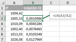
in column A - the price of the abstract asset ABS / USD, $$$p_ {i}$ .
Column B contains the natural logarithm of the private $$$p_ {i}$ and $$$p_ {i-1}$ .

Lognormal distribution describes a price series, the derivative of which, obtained as the natural logarithm of the quotient from dividing the current value with the previous one, has a normal distribution. Complicated. Let me explain with our example: if the values ​​in column B are distributed according to the normal law, then the values ​​of column A describe a log-normal distribution.

How do we get a “lognormal” price series? MS Excel, which I have already used for the example, is able to generate random numbers that have a uniform (alas, not normal) distribution. There is a simple method by which we can obtain a series of normally distributed CBs from uniformly distributed CBs. The technique is called the “inverse function method”. Without going into details of the method, I will note the following important aspect of it:

• the method of the inverse function allows you to get CB with an arbitrary, given function (table), the distribution law, getting at the input CB, evenly distributed in the range from 0 to 1.

We need the inverse integral (as it is also called, cumulative) normal distribution function. This is in Excel: the “NORM. OBR” function.

The NORMAL OBR function takes values: probability, mean, standard deviation.

• Probability is the very value from which we build our function. Strictly more than 0 and strictly less than 1. We will generate 999 values ​​from 0.001 to 0.999 with a step of 0.001 in column A. The values ​​from column A and go to the input of the NORMAL CODE function.
• The average is the mathematical expectation of our SV. Let me remind you, we are generating a value proportional to the dynamics of our price asset ABS / USD. Positive values ​​correspond to price increases ( $$$p_ {i}> p_ {i-1} \ implies ln (p_ {i} / p_ {i-1})> 0$ ), negative - fall. If we set the “average” parameter to greater than zero, our asset will most likely grow (the programmer says: we will spend a million iterations and are guaranteed to see the final price that exceeds the initial value). Our choice is an average of 0. That means the “neutral drifting” price of ABS / USD.
• Standard deviation. About him, too, will be discussed later. The value that characterizes the volatility of our asset. Take it equal to 0.5% or 0.005. Which roughly corresponds to the change in price per day by ± 0.5% on average.

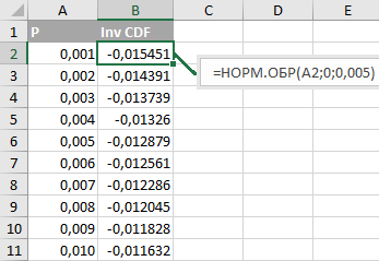
How to interpret this data? Take the first pair of numbers:

“CB will take a value of -0.015451 or less with a probability of 0.001 (0.1%)”.

The second pair: “CB will take the value -0.014391 or less with a probability of 0.002 (0.2%)”. Etc.
Inverse function method: we randomly select a number in the range from 0 to 1 (column A) and find the corresponding value of the inverse of the cumulative distribution function (column B). Or, in our case, simply randomly select a number from column B.

Ie, choose the value of N in the range from 0 to 999 and read the contents of the cell $$$B_ {n + 2}$ :

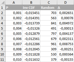
• Cell formula B2: = NORM. OBR (A2; 0; 0.005)
• Cell formula: C2: = CASE (0; 999)
• Cell formula D2: = DVSYL (CLUTCH (“B”; C2 + 2))

So we got a normally distributed random variable with a mean of 0 and a standard deviation of 0.005.

There can be any number of values ​​in column D. We will need 3650 values ​​- we are going to simulate the daily price changes of ABS / USD for 10 years. It remains to generate the actual price of ABS / USD.

In column D we have a series of values ​​of ∆, and ∆, by the formula of a lognormal distribution, is defined as

$$

$$∆_ {i} = ln (p_ {i} / p_ {i-1})$$

Hence, the ABS / USD prices, the following and the previous ones, will be related by the function.

$$

$$p_ {i} = p_ {i-1} * e ^ ∆$$

Transfer the column D to the new sheet, copy it, and then paste the values ​​starting at cell A3.

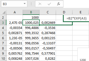
Now we indicate the initial price of ABS / USD equal to 1000 (USD for 1 ABS) - enter “1000” in cell B2:


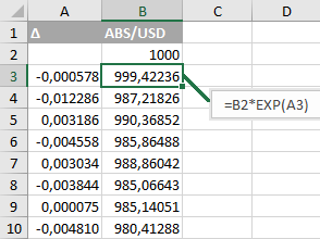
In cell B3, enter “= B2 * EXP (A3)” and copy this value into all subsequent cells - B4: B3652.

This completes the preparation of the initial data, finally. Column B contains the price range of our benchmark ABS / USD asset. A series with lognormal distribution characteristics with a standard deviation of 0.005 (0.5%). I got the following values:


There is no guarantee that if you perform exactly the same calculations in MS Excel, you get exactly the same values, since the source data is a random variable. And yet - you see, the schedule is quite like a stock quote?

The calculation of the premium formula BB

Since we have “reference” data, we will carry out a “reference” calculation. We consider the premium for the “vanilla” European CALL option:

• The current price (S) is 1000,
• Strike (X) is equal to 1000. Strike is equal to the current price, such option on slang is called “vanilla”,
• expiration after 30 days (T),
• transaction volume - one contract.

Our ABS tool is not a stock, not a bond, or any other security. No dividends for the possession of ABS owner is not entitled.

The same formula is the formula for calculating the premium for a European Call option (value C):

$$

$$C = SN (d_ {1}) - Xe ^ {- rT} N (d_ {2})$$

$$

$$d_ {1} = \ frac {ln (\ frac {S} {X}) + (r + \ frac {σ ^ 2} {2}) T} {σ \ sqrt {T}}$$

$$

$$d_ {2} = d_ {1} -σ \ sqrt {T}$$

Let us analyze the parameters of the formula.

• S and X are already known to us - the current (1000 USD) and strike (1000 USD) asset prices, respectively.
• T - time to expiration, expressed as part of the year. For example, our ABS contract is trading 365 days a year, like cryptocurrency contracts. Expiration will occur in 30 days, therefore, T = 30/365 ~ 0.082. Another example is an option on EURUSD on the Chicago stock exchange, trading approximately 265 days a year. We count the number of trading days before a specific date - before the expiration day. Let's say we counted 23 trading days. In this case, the parameter T will be equal to 23/265 or approximately 0.087.
• r - risk-free interest rate. As we have already noted, for the asset ABS, it is equal to 0.
• σ (sigma) is the historical volatility of an asset. This will require a small digression.

Historical volatility

For volatility, we take the standard deviation (RMS), recalculated for the annual interval. Let me give you another formula from Wikipedia:

$$

$$S_ {0} = \ sqrt {\ frac {1} {n-1} \ sum_ {i = 1} ^ {n} (x_ {i} - \ overline {x}) ^ 2}$$

How do we calculate the standard deviation of ABS / USD prices in MS Excel?

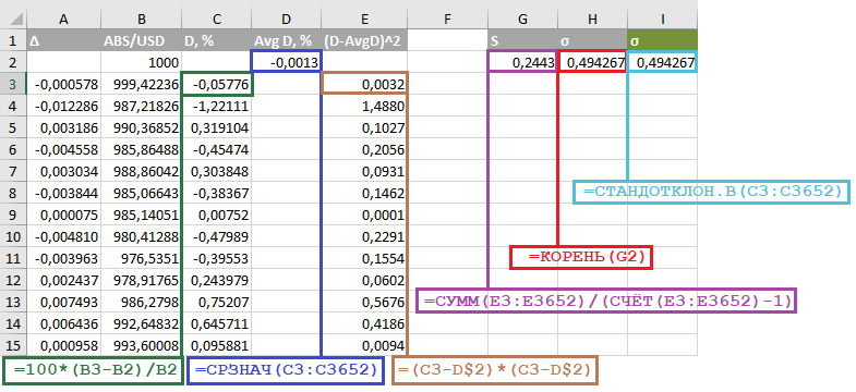
• Column C contains the difference between the current and previous values ​​of the ABS price, divided by the previous value and multiplied by 100%.
• Cell D2 contains the average of column C.
• Column E contains the squares of the difference between the price deviation (column C) and the average value of the price deviation (cell D2, the second line is “fixed” in the formula by the symbol $).
• Cell G2 is the variance, the sum of the squares of the deviations divided by the number of values ​​minus 1 (SIC!).
• Finally, the H2 cell contains the required RMS, the root of the variance (G2).

Some of the calculations can be skipped: it is enough to calculate the C column (deviations in percent) and use the Excel function to find the root-mean-square (standard) deviation — as we defined in cell I2 — the STANDOCLON.B function.

It remains to recalculate the standard deviation (σ) value for the interval of one year. Our ABS / USD is trading 365 days a year. The σ value calculated for one day should be multiplied by the square root of 365:

$$

$$σ_ {Y} = σ \ sqrt {365} = 0.4943 \% \ times19,105 = 9.443 \%$$

Where did the square root in the formula for recalculating the daily value of the standard deviation per year come from? Interested address on the Internet, look for a model of random walk, random walk (RW).

Excel premium calculation

Now that we have defined all the parameters of the Black-Scholes formula, we will enter their values ​​and functions in Excel:


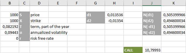
I note right away: I indicate the values ​​of T and σ in absolute terms, not in percentages.

• The formula of the coefficient is d1 = (LN (B2 / B3) + B4 * (B6 + B5 * B5 / 2)) / (B5 * ROOT (B4))
• d2 = H2-B5 * ROOT (B4)
• N (d1) = NORM.DIST (H2; 0; 1; TRUE)
• N (d2) = NORM.DIST (H3; 0; 1; TRUE)
• Finally, the premium of the CALL option: = B2 * DEGREE (2,71818; -B7 * B4) * K2-B3 * DEGREE (2,71818; -B6 * B4) * K3

The “fair” premium for the vanilla European CALL option ABS / USD with strike 1000 and expiration in 30 days was $ 10.80 for one contract.

Calculation of premium for “abnormal” price distribution

Above, it was stated that the price model B-SH is adequate for the lognormal distribution of the price series. But how close is the “real” market in its characteristics to the law-like distribution of CB? More precisely, how far is the market from it?

Our hypothetical asset ABS / USD is characterized by a normal distribution of logarithms from private neighboring (current and previous) prices. The graph of the probability density of the occurrence of large and small price deviations (logarithms) has a classical for normal distribution form, approximately like this:


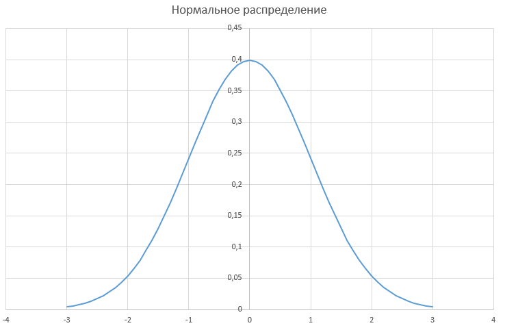
In other words, it has the shape of a bell, with a “steep” apex and “shoulders”, or “tails”, rapidly approaching the abscissa as it moves away from the mean value (0).

What empirical observations would be appropriate for the real market for these very “tails” of the normal distribution?

Large price deviations are possible, but have an extremely low probability. For the chart above, we can say that the price deviation of + 2% or more has a probability of 5%. And the price deviation of + 3% or more already has a near-zero probability - some insignificant fractions of a percent.

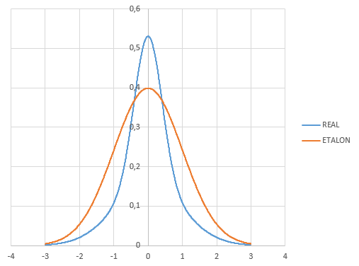
The “real” market has a slightly different behavior. Specifically: the majority of price changes lie in a rather narrow range, while, however, the probability of significant price fluctuations is significant. The graph of probability density of price deviations for the “real” market will look like this:


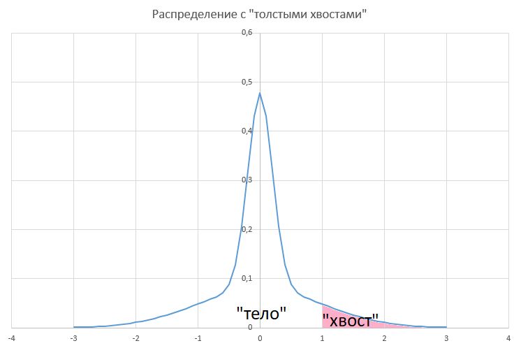
Will the fact that the characteristics of the distribution of daily price deviations for the “real” market differ from the B-Sh model affect the accuracy of the calculation?

Obviously will affect. The question is - how much will the B-Sh formula be mistaken in its assessment of the “fair” award?

Modeling "real" prices

Now my task is to generate a new price range. The price series, the logarithms of the private neighboring prices in which obey a certain “abnormal” distribution - a distribution that is distinguished by “thick tails”. Moreover, I will complicate my task a little.

The final price series should be characterized by the same amount of historical volatility as the ABS / USD price range that we built earlier.

For example, let me give you two curves of the density of the distribution of CB: the normal distribution (the brown line) and the “real” distribution (the blue line) are what we want to get. With thick and long tails:


In the normal distribution, we can vary one parameter - the standard deviation (σ). Here are two graphs of the density of the normal distribution with σ equal to 1 and 0.4, respectively:


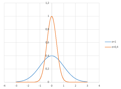
Both graphics are not exactly what we would like. The thin “body” of the graph for the parameter σ = 0.4 is close to the desired one. But we would like the “tails” thicker. In other words, a large percentage of deviations are concentrated in the vicinity of the mean value (0), with still significant probability of large (2% or more) price deviations.

Solution: add up two graphics. I will get the very dependence that I cited above in the figure as the “real” probability density of the price distribution.

Now we have added the values ​​of the density function of the normal distribution. How to build a distribution, the density of which will correspond to the sum of two normal distribution functions with parameters σ = 1 and σ = 0.4?

Obviously ( corrected ):

1. add two (inverse) integral density functions of the normal distribution,
2. substitute the argument in the resulting function - a uniformly distributed CB.

I will do about the same calculations as before, when generating a number of ABS / USD. But now I’ll fill the two columns with the “NOR.OBR” function. The resulting value should have an annual standard deviation equal to 9.44% - as in the previous example. I will achieve this by conducting several iterations of the selection of parameters, since the result (generated sample) is non-deterministic:

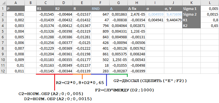
• Columns C (R1), D (R2) contain the inverse normal distribution function with parameters 0.005 and 0.0015, respectively.
• The column E (R) is the weighted sum of these two values ​​— 0.8 x R1 + 0.65 x R2.
• Column F (RND) is a random number in the range from 2 to 1000.
• Finally, the column G (∆) is a cell randomly selected from the column E (R). That distribution, which we sought.

It remains to apply the formula to the series obtained:

$$

$$x_ {i} = x_ {i-1} * e ^ {∆_ {i}}$$

The sum of two normally distributed random variables is copied to column A. In column B, as before, we multiply the previous price value (starting from 1000) by the exponent from CB from column A.

As a result, I got the following price chart for WRD / USD:


The premium for the CALL option for WRDUSD on the same terms of the contract that we have previously calculated will remain unchanged, since the parameters in the B-Sh formula have not changed. Let me remind the numbers: the premium for vanilla European CALL-option WRD / USD with strike 1000 and expiration after 30 days was $ 10.80 for one contract.

We have two assets, the price dynamics for which is expressed by different laws:

	ABS / USD	WRD / USD
Price distribution law	lognormal distribution	"Real" distribution
Award according to the formula BC	$ 10.80	$ 10.80
“Fair” award	?	?

At this stage, MS Excel does not already have enough capabilities; it's time to move on to programming. To be continued…