Time is money. As we taught Yandeks.Taksi accurately calculate the cost of the trip

Any of us before buying a product or service tries to find out the exact price. It is clear that sometimes stories happen when the final cost greatly exceeds the planned one. And if with repair of the car or apartment it already became habitual, in other cases the difference between expectation and reality is rather annoying.

Until recently, the cost of travel in a taxi was also floating. Even online services calculated the amount only approximately - the final cost was formed only at the end of the journey. The fare typically includes three components: the cost of landing (sometimes with kilometers and / or minutes included), the cost per kilometer, and the cost per minute. Of course, it was possible to calculate the approximate price for a trip before, but in the end it could change due to the fact that, for example, the driver stayed in a traffic jam on the way. It is clear that passengers did not always like it.

It seems that there is nothing easier than using the data of the router in Yandex.Navigator and the data of traffic jams so that Yandex.Taxi from the very beginning would calculate the exact price that would not change at the end of the trip. But in fact, the cost is influenced by a huge number of factors, not just the tariff. It is important not just to be able to count it. On the one hand, the cost should be attractive to the user, and taking into account not only the current situation on the road, but also, for example, traffic jams, which are not on the route yet, but which will soon arise. On the other hand, the price should be such that drivers do not lose in earnings, even if the path from point A to point B is longer or longer than planned. In this article, we will describe how you solved the problem and how you looked for a balanced algorithm that benefits all participants of the Yandex.Taxi platform.

Route and time

In order to be able to calculate a balanced trip cost, we had to learn how to accurately predict the length and duration of the route. Let's see how our router works at all.
')
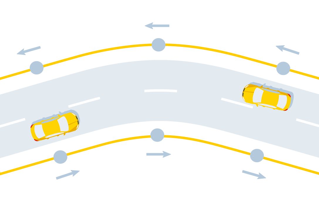
This is a rather complicated system that builds a route from one point to another on the basis of another simpler system - a road graph. The graph looks as natural as you probably imagine it to be: each road corresponds to one or several edges, and the intersections and branching of the roads are located at the vertices. This graph is directional (as the roads are also directional).

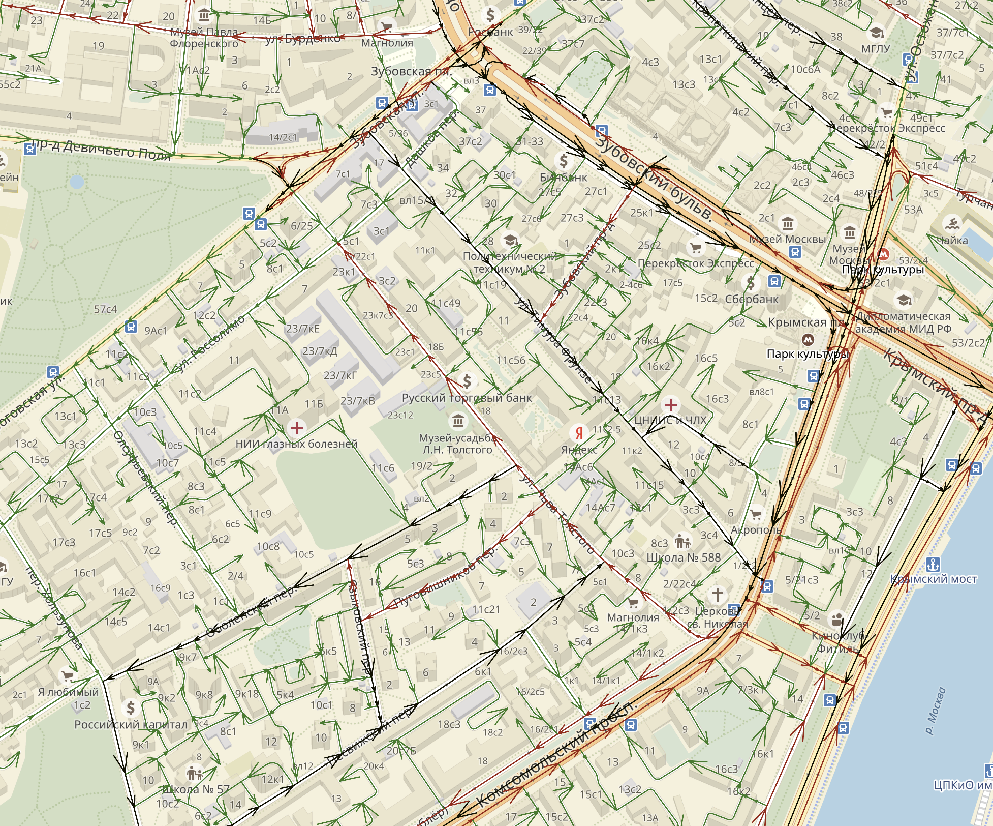
_{^{This is what a road graph looks like in the area of ​​the Moscow office of Yandex}}

The most important characteristic of the edges of the graph is the average speed of movement along them at the moment. It depends on the current traffic situation and the rules of the road (for example, speed limits). Every second we receive tens of thousands of impersonal signals — GPS tracks — from users of Yandex geoservices, aggregate them, and then, by filtering and interpolating, we make the signal better and less noisy. At the final stage, we calculate the current edge speed in real time (for more details on how Traffic jams work, see here ).

The address — the “top” of the virtual graph — consists of the edge of the road graph and the direction of motion along it:
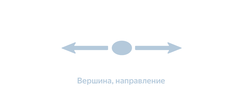
What happens when you book a trip in the app? We send a request to the router in order to find the best route from the landing point (A) to the destination (B), which is specified in the order. The router, in turn, projects a point A onto the graph in order to find its “address” —a combination of an edge and a direction. The same thing happens with point B. And the first feature of the system is already manifested here: the process of determining the shortest path occurs not in the original, “natural” road graph, but in a certain “virtual” one. Its vertices are no longer intersections, but the very "addresses", and the edges - not the streets, but "maneuvers", that is, transitions from one "address" to another.

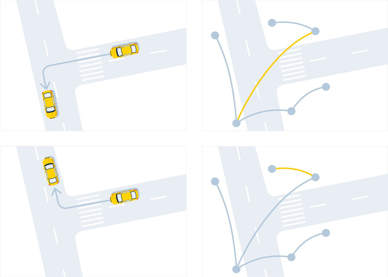
_{^{Representation of the same trajectory of movement in the road (left) and virtual (right) graphs}}

_{^{A straight line movement can also consist of virtual graph maneuvers: for convenience, the long road turns into several edges when digitizing.}}

As we remember, our task is to find the optimal route, while, of course, the final “physical” route will be completely unimportant whether we built it in a “natural” graph or a “virtual” one. But first you need to decide what is optimality. On the one hand, it is obvious that in the city it is the fastest way from A to B. On the other hand, sometimes a difficult route through small streets and bypassing major highways, although it saves 2 minutes, but due to the large number of turns it turns out to be significantly "More expensive" for the motorist. Therefore, to begin with, we defined a function that sets the “cost” of the maneuver and decided to optimize it using machine learning.

The simplest example of such a function is the length of the edges that make up the maneuver, divided by the average speed of movement along these edges, the so-called “geometric time”. This metric is good in its simplicity, but it often does not take into account a number of features of a particular maneuver. Take for example the left turn. Obviously, to make it from a secondary road at an adjustable intersection is not at all the same thing as turning onto a ramp, moving along a highway. The characteristics of each individual situation can significantly increase the time to complete the entire maneuver, and in order to take them into account, we decided to describe each maneuver with a set of attributes: the length of its edges, the geometric travel time, functional classes of roads, the presence of a dedicated public transport strip, and so on. Here, “signs of the future” naturally arose: for example, we can calculate in advance the time for passing a maneuver, taking into account traffic jams that will arise by the time we approach this maneuver.

As a result, we got more than 70 different signs affecting the “cost” of the route, and their number is constantly growing, because we are constantly adding new signals that can become signs and help in our task.

Another feature of our approach is that we have divided the original task into two: building a route and specifying the travel time on it. We called these models “route” and “time”, respectively, and it is worth telling in more detail how they differ from each other and why we need two models.

The route model is used to select the optimal path from point A to point B from a variety of options, based on the length of the route and travel time on it. The catch here is that the routing model must produce an answer very, very quickly, because after it, the system needs time to use these calculations in a further process chain. Say, 100 milliseconds for a calculation of 1000 maneuvers is too much, you need an order of magnitude less. The route model should be as cost-effective as possible in terms of computation, so it takes into account a reduced set of features. But when we already have an optimal route - we want to know the time to travel through it as precisely as possible, and here we are not so connected by speed, we can afford 100 milliseconds.

For this, there is a time model, the only task of which is the specification of the travel time for an already chosen route. The time model takes into account the full set of features for each maneuver, as well as user request parameters from the application: the current local time and various route macro-characteristics — for example, the over-run ratio (the ratio of the actual route from A to B to the distance between these points in a straight line). At the exit, the time model gives the updated travel time.

To summarize: our initial task “how to most accurately build a route and predict the time to travel on it” has been reduced to several steps. First, we moved from a “natural” graph with vertices-intersections and edges-streets to a “virtual” graph, the edges of which are maneuvers, that is, transitions from “address” to “address”. Each of these maneuvers we described with a set of more than 70 signs. Secondly, in order to optimize the operation of the router, we decided that there will be two predictive models: the route one, which is quick but rough, chooses the right route from the set of possible ones, and the time one, which specifies the travel time by the optimal route. Now how these models work.

Models

Despite the fact that both the route and time models are very different from each other, they, in fact, have a similar task - to calculate the time of travel along the route. The key difference is in the complexity of the calculations used, that is, in quantitative rather than qualitative factor. At the same time, since the models have the same task, then the approach from the point of view of their training is the same. We can take only one model — the time model — and then remove “all unnecessary” from it (for example, unnecessary features) and thus obtain a more lightweight route model.

This approach turned out to be advantageous not only because it unified the machine learning method, but also for other reasons, including because the training of the time model is a classical task, as they say, “from the textbook”. We have a huge base of travel histories, that is, there are a lot of “route-time” pairs that can be used as a sample for some kind of machine learning method. It is more difficult to train the route model, because we cannot force all drivers to ride along all the variants of routes from point A to point B in order to compare which one is faster. As a result, at the first stage, we focused precisely on training the time model.

The first idea was simply to use a linear model over the sum of signs of maneuvers along the route, and to take the actual travel time as the learning goal. This approach has a characteristic of the problem - linearity itself. Indeed, the time calculated in this way for a route consisting, for example, of two maneuvers, is equal to the sum of times calculated for each of the maneuvers separately. There were no difficulties with the interpretation of various signs, which is always pleasant: if the weight with a sign is large, then the sign is significant.

Nevertheless, despite a lot of advantages, the very first attempts to train this model turned out to be disappointing: the results were slightly better than “geometric time” because we lost a lot of information embedded in categorical (that is, unnumbered) signs of maneuvers - for example, the functional class of roads , the shape of the ribs, the level of the road above the ground and others remained "overboard".

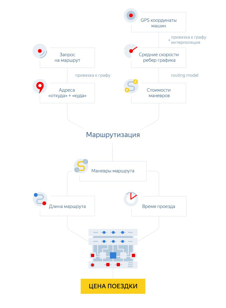
Here is how the price of the trip is calculated at the time of booking:


As we know, taking into account categorical variables is always a difficult task, it was not for nothing that the whole CatBoost was invented . And yet we tried to solve this problem by using a technique similar to N-way-split, which is used in decision trees.

We take into account that, according to the classification of People’s Maps, the roads are divided into 9 functional classes , and there are also 5 types of design features: two carriageways, a roundabout, a congress, a backup, a U-turn. In addition, on the road or there is a traffic light or it is not - these are two more values. Total we have 9x5x2 = 90 combinations. Now for each such combination of categorical signs, we will separately take into account the remaining signs, that is, we will initially divide our sample into 90 independent fragments. Because of this fragmentation, we in total received several thousand signs, because in essence we examined each of them 90 times - for each separate combination. Even with the large training samples, such “animation” led to the fact that the model began to quickly retrain. Partially, this problem was solved by L1-regularization (it, unlike L2, is able to level the influence of the signs, zeroing the weight of them), but in the end, by the totality of problems, the approach had to be considered a dead end. True, there were some good news: such a time model could already be used as a route one, because it had linearity in individual maneuvers, which means we were moving in the right direction.

And yet, the problem remained: how to cope with so many signs? Yandex has Matrixnet , a machine learning algorithm based on gradient boosting of decision trees, which successfully copes with hundreds and even thousands of attributes. To begin with, we tried the “head on” approach and trained the Matriksnet on pairs of “route - real travel time”. Such a method immediately gave a good result, and further work on increasing the number of features and fine-tuning the algorithm hyper parameters helped to get a noticeable increase in the quality of prediction. But, despite the instantaneous “exhaust”, caused simply by the power of Matrixnet, there were also disadvantages:

• It became difficult to interpret the results, because in the case of gradient boosting over trees, we are working, in fact, with a black box. It is no longer possible to simply interpret various signs depending on their weights.
• The linearity disappeared from the model - it’s impossible to split the route into 2 pieces, apply the model to them, add up and get the same number as for the entire route.
• This model could not be used as a route one, because we trained it on the routes as a whole, and not on individual maneuvers.

That is, for our tasks, the use of Matriksnet "in the forehead" did not fit. As a result, we were left with two different models, each of which was good in its own way, but also something bad. In this paradigm — the linear (and threatened to retrain) route model and the time model based on Matrixnet — we tried to develop for a while, but the soul wanted some kind of universal solution. And it was found.

"Linear MatrixNet"

As it usually happens, the idea, when it came to my head, turned out to be simple to tears: to apply Matrixnet to individual maneuvers, not to the whole route, but to take the following difference as a function of the error: sum of time values ​​by route maneuvers minus target travel time .

$$

$$\ sum \ limits_ {r \ in routes} (T_r - \ sum \ limits_ {m \ in maneuvers} F (f_m)) ^ 2,$$

where T is Target, f are attributes, F is an optimized function.

Although this function is very similar to the task of ranking in the search (optimization of search results as a whole), there was no such a tool of the Matrixnet among the finished ones, so we had to implement it ourselves.

After some agony of picking the right pace of training and the number of trees, we managed to get a model that almost did not lose to the “pure” Matrixnet in quality, but it was linear. This made it possible to use it as a routing model, and also opened up access to the easy use of categorical features by digitizing them and using CatBoost.

results

The whole story took a lot of time, but ultimately we got a model that simultaneously met all the requirements for speed and gave the necessary accuracy in estimating time. It was this last characteristic that made it possible to accurately calculate the cost of a taxi ride in advance, and not to change it at the end of the journey.

The last question - what results did we get, is there anything to compare with? Of course, a complete answer would require a discussion of a variety of factors and quite serious analytics. But we can give some very simple estimates.

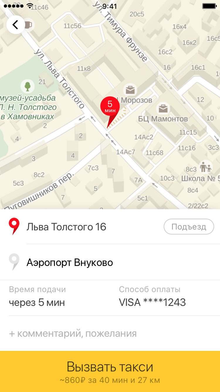
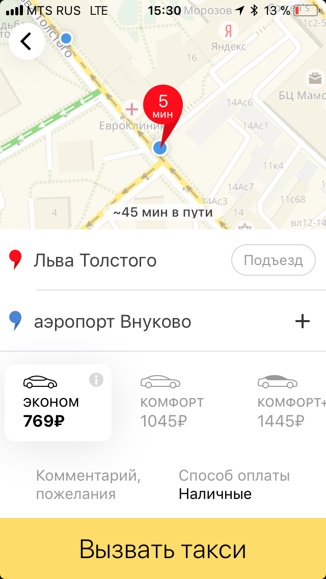
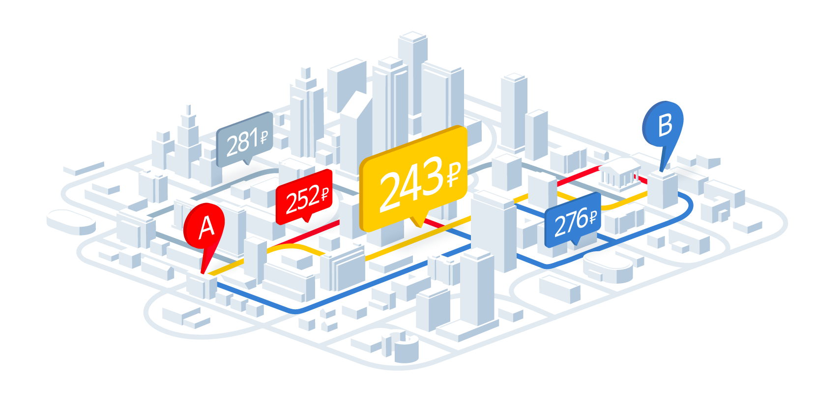
_{^{"It was - it became." On the left - the old version of the application with an approximate calculation of the cost of the trip. On the right - the current version with the exact price of the trip in different fares.}}

Obviously, showing the exact price of a trip in the Yandex.Taxi application even at the time of booking is in itself a significant advantage, which makes the service transparent for users, so here we took little risk. The only thing that turned out to be difficult is to explain that if a person arrives at the wrong point B, which he indicated when ordering, then the whole trip is recalculated using a taximeter, because in such cases our calculations are meaningless. But that's another story. Since there are not many such cases, the majority of our users appreciated not just the display of the final price before the trip, but also the fact that it did not change at the end of the trip, even if the taxi was in a traffic jam or the driver was driving around. And of course, they began to point out point B more often, realizing that only in this case they get such a calculation.

As we said at the beginning, if our algorithms worked poorly and made the price good only for the user, this could lead to a significant loss of earnings for drivers and, as a result, to their outflow. After the price began to appear even before the trip, the number of orders began to grow actively - many people for whom the exact cost is critical, it became psychologically easier to use Yandex.Taxi. The increase in orders has led to a significant increase in the utilization of taxi cars - that is, to share for the work shift, when the driver is carrying a passenger or driving to order, and not wasting time. It also happened due to the fact that growth has improved the work of other service technologies - for example, a chain of orders. This is an algorithm that begins to look for the next client before the driver takes the previous one - and is looking for him in the area where the driver will soon arrive with the passenger.

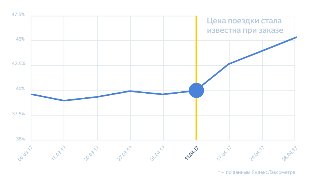
_{^{The growth of recycling machines in Moscow and the region.}}

Thanks to the increase in recycling, the most important indicator for a driver is earn per hour, the average earnings per shift hour: according to our estimates, by about 15–22% on average in Russia. Although some cities turned out to be real champions, this indicator grew even more there.

Ahead of us are waiting for many small and major improvements of the model, such as connecting CatBoost, about which we will definitely tell.