Convolution network in python. Part 3. Application of the model

This is the final part of articles on convolution networks. Before reading, I recommend that you familiarize yourself with the first and second parts, which examine the layers of the network and the principles of their work, as well as the formulas that are responsible for teaching the entire model. Today we will look at the features and difficulties that can be encountered when testing a convolutional network written manually in python, apply the written network to the MNIST dataset and compare the results obtained with the tensorflow library.

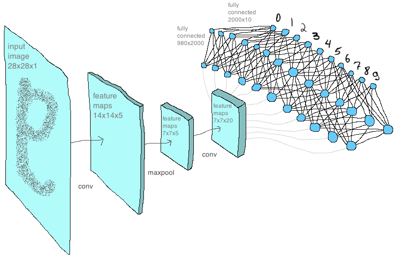
Now you can see the basic concept of the network, the structure of the layers and their sequence. Below I presented it in the way I implemented it in the code - each layer as a separate function (you can remove or add new layers as an experiment, swap them or write your new layer):

Direct passage through the network

1) The first layer of the convolutional network
2) Maxpooling Layer
3) The second layer of the convolutional network
4) Adding all feature maps to one vector (this is not quite the “full-fledged” layer, but nevertheless occupies an important place here)
5) First layer of fc network
6) Second layer fc network
7) Calculation of the loss function
')
Reverse passing through the network and updating the parameters (we go through all layers in the reverse order)

8) Backprop through loss
9) Second layer fc network
10) First layer of fc network
11) Expanding feature maps from a vector (also not a “full-fledged” layer)
12) The second layer of the convolutional network
13) Maxpooling Layer
14) The first layer of the convolutional network

Of course, one should not expect this model to work faster than an optimized library for machine learning. But after all, the ultimate goal is not to write a quick implementation, but to understand how the library works, to learn how to build a neural network on the lowest level, and after previous articles with the considered principles of operation and formulas, all that remains is to write code. Further an example of such code.

model.py - all major functions that make up the network are stored here. Many of the functions we have already covered in past articles.

np_mnist_train_test.py - the network itself and the input parameters for it. The network is built from the functions defined in model.py, and it looks literally in the same way as the 14 points that we identified at the beginning of the article:


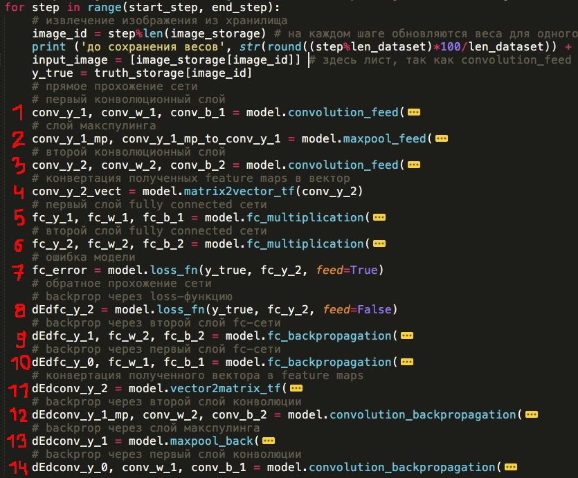
(I hid the function arguments, in expanded form everything looks scary)
But before going on to describe the results, I would like to dwell on another. Applying the written model to the data, I saw that she was trained and everything passed without errors. However, I wanted to be sure that the network is working correctly, that all internal calculations are correct. And the most obvious solution was to compare this model with a similar architecture at tensorflow, using, for example, MNIST as a dataset.


It was much easier to write a network to tensorflow, in fact, I just took this option from the tensorflow manual and slightly modified the parameters. It turned out this model:

tf_mnist_train_test.py

To make sure that the results of both models are the same, you must first make sure that their starting weights are identical. Here was the first difficulty - I could not fix the seed separately for numpy and tensorflow so that the initial randomly generated weights matrices coincide. I came up with this trick: create weights in tesnrflow and feed them into both models. But it seems to me that this issue could be solved and somehow easier. But in the end, it looks like this:


To extract the weights from the tensor in the order that tensorflow sees them, that is, in the manner in which they are used in further work inside the library, I used the code above. As you can see, everything is not quite trivial: the tensorflow tensor had to go through a couple of Resapes and transposition so that it could be used in the numpy model. Also for this reason, some other functions had to be rewritten. For example, the function of combining all feature maps into one vector is when many feature maps form after the convolution layers and it is necessary to vectorize them for submission to the fc network. After we have broken the tensor into matrices using the above method, we cannot combine the matrices into a vector anymore if we want it to look the same as inside a tensorflow. And in order to achieve this, we must do the following:


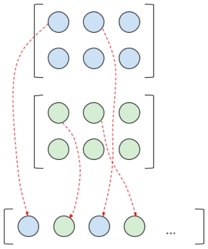
Accordingly, when in the case of the reverse propagation of the error, we went through fully connected layers, we will have a vector of gradients, which we need to “straighten” back into the feature maps. This is done as in the picture above, only in the opposite direction. Of course, if the goal is not to compare the results of calculations of numpy- and tenosorflow-models, these functions can be written in a simple way. Here, in fact, I described what the matrix2vector (matrix-to-vector) and vector2matrix (vector-to-matrix) functions do in model.py.

The following: feature maps are viewed as channels of one, so to speak, image, and not as image independent of each other. Initially, I assumed that if we want four feature maps at the output, then there should be four cores, but it all turns out a little differently. Since all feature maps of the previous layer are considered as one image with multiple channels, then to get only one map on the next layer, you need to create as many weight matrices as there are channels on the previous layer (respectively, for two maps, twice as many weight matrices). Then get the appropriate number of “intermediate” maps and put them into one - this will be the desired feature map. Let's say, if there were two cards on the previous layer, and we want to get four on the next layer, then it will look something like this:


When adding, “intermediate” maps of signs seem to be shuffled to produce a “final” map, but if you look closely, it is clear that only those “intermediate” maps of signs that originate from different channels of the original layer are added to the final maps. Maybe thanks to the image below it will be better understood:


Here we want to get two feature maps from one RGB image. And I’d also note: during the reverse propagation of an error, those “intermediate” cards are not involved at all: they don’t exist at all in the understanding of the program. Each matrix of weights and a feature map from the previous layer are tied to the corresponding “final” maps of the next layer.

The next feature of tensorflow calculations was the fact that inside the tf.nn.conv2d function, cross-correlation actually occurs and this is even written in the tensorflow manual :

It is strictly speaking that they have been strictly speaking. For details, see the properties of cross-correlation.

But this did not become a big problem, since in my implementation for numpy it is enough to change True to False. Here is an example of code with which you can make sure that it is cross-correlation that is used:


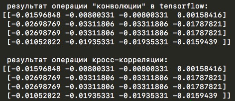
The same demo code contains another interesting detail of calculations in tensorflow. Inside the library, during the convolution operation, the central element of the convolution kernel sometimes changes. Usually it is in position (0,0), but for the 3 by 3 core it moves to the central position (1,1) (and maybe, in fact, the opposite is true and the “usual” position is exactly in the center (1,1) and the core is relative to it and moves to the upper left corner ...). If, for this kernel, we set the stride to two, then the central element in tensorflow will again move to the zero position. The logic is, as it seems to me that with the dimension of the input matrix 4 by 4 pixels and a step of two pixels, we expect an output matrix of dimension 2 by 2. And this is exactly what happens, but only if the central element is in position (0.0 ), if the central element is in (1,1), then the dimension of the output matrix under such conditions will be three by three pixels. This is due to the fact that the core with the central element in (1.1) manages to perform more calculations before it is “hidden” outside the input matrix. Here, look at the picture below:


And thus, if the code written from scratch does not take into account the possibility of choosing a central element, then one could never understand the reason for the difference of results from tensorflow.

So, finally, we dismantled all the nuances that led to differences in the results, we took into account all this in the from scratch model and we can compare the losses of both networks: the first one implemented using numpy, and the second - the library at tensorflow.

Next, a little about network architecture. On the first convolutional layer, I used a 2x2 pixel core (and the central element in the zero position) with a step equal to two, this layer produces five feature maps of 14x14 pixels (that is, two times smaller than the original mnist images of 28x28 pixels). These cards are fed to the second layer with the core already three by three pixels and one step (which, I recall, leads to the displacement of the central element, in fact, in the center of the core), and at the output of 20 feature maps of the same dimension. Then a layer of max-cooling reduces the dimension of maps to 7x7 pixels. Then the cards add up to a vector. Next is the hidden layer of a fully connected network with two thousand neurons. On this layer in the weights matrix, almost two million (7 x 7 x 20 x 2000 = 1 960 000) elements are obtained! And then already 2000 neurons are connected with 10 output neurons responsible for the number of classes: that is, 10 digits that the network must learn to predict. All these parameters are listed in a dictionary called model settings, which is located inside the np_mnist_train_test.py file:


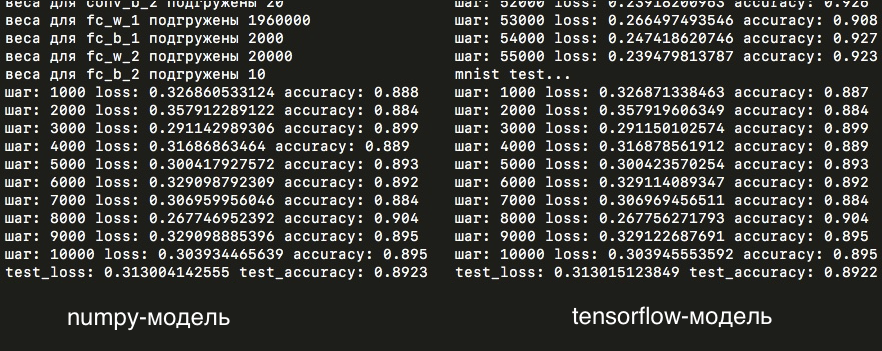
So, let's try to run both models and compare the results: loss and accuracy, averaged over each five images:


As you can see, the losses in almost completely coincide, which means that all the calculations within the manually assembled model and the model written in tensorflow are at least very similar.

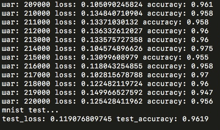
After a day and one epoch of training (that is, 55 thousand iterations of the forward and backward passage of the network), we got such graphs for loss and accuracy:


And on the test sample, accuracy is 89%:


As you can see, the loss for the numpy-model team on the test and training samples is very similar to the results of the network by tensorflow. The difference in accuracy on the test sample after one epoch of training is only one image per ten thousand! But nevertheless the weights matrices themselves differ in thousandths (whereas there was no difference in the first stages of training) - the difference is most likely due to the different accuracy of calculations in numpy and tensorflow: float32 and float64, or other unaccounted nuances that make minor differences in model calculations.

Accuracy 89% was achieved after just one era. But after already four epochs on the same model, the results on the test sample would have been significantly higher - 96%. But I tried it only at tensorflow, on the numpy-model further training took too much time, but in general it can be concluded that the chosen architecture is not as bad as it could be!


To be precise, one epoch on the numpy-model took about 15 hours on an old laptop. On the model assembled using tensorflow, the same era passes in just 7-8 minutes. That is a difference of 120 times! What does it take all the time in the manually assembled model and where is the bottleneck? To understand this, just look at the timeline that each function takes in the numpy-model (total for forward and backward passes through the network):


As you can see, almost all 15 hours several convolution cores are trained. That is why in the model parameters I have so few feature maps at the output of convolutional layers. The full-connected layers take almost no time (especially the second fc-layer with a smaller number of parameters), since inside there is an optimized multiplication of the numpy-matrices, whereas the convolutional functions were written on the basis of formulas and the literal “movement” of the kernel along the matrix. The calculations of tensorflow are much more optimized and the convolutional layers are also presented in the form of matrix multiplication. Here you can read more.

I tried to study the model with “non-standard” parameters - the operation of convolution instead of cross-correlation and the central elements in the position (1.0) for the first layer and (1.2) for the second convolution layer. The results were worse, but with further training, it would probably be aligned with the usual parameters. Of course, I could no longer compare the calculations with the tensorflow model, since it is not possible to change the specified central element to any other or cross-correlation to convolution for any layer of the convolutional network (in general, it is unlikely may come in handy someday). Interestingly, accuracy at the very beginning began to grow sharply upwards, but after that it was already far behind the “normal” model.


Of course, the numpy-model is not suitable for real calculations and tensorflow or other machine learning libraries should be used. I can’t say that I’m absolutely sure that there are no errors in the python implementation, that all the subtleties and nuances of training that are definitely in tensorflow are taken into account. But the main thing is the time of study. The fact that python takes two hours, to tensorflow - just a minute.

To improve the results obtained on MNIST, you need to use more convolutionary layers, generate more feature maps for the network to adequately extract features from images (all this, of course, will seriously affect the learning time if you use the model on numpy). You should also use the batch in more than one image, the classical SGD optimization method should be replaced with, for example, Adam (which can be read here or here ). The results we obtained in the article are, of course, not impressive (the leaderboard can be seen here ), but it is clear that the model, written literally according to the formulas, really learns, works. If you want to reproduce the test results, or continue your training, we have cnn_weights_mnist.npy weights for the numpy model in the git repository.

This is the end of the article on convolutional networks. Well, if now you already have an idea about the internal structure and mathematics, which stands behind the networks and is hidden inside the library for machine learning. I tried to tell everything as simple as possible and sort out all the formulas so that there were no questions left, and I hope that these articles save someone time. Well, that's all, thanks for reading to the end!