Quantum computing: annealing with switches and other fun
In the previous article, we started a story about quantum computing and compared them with ordinary ones. Today we dive deeper into their technical features and tell you how it is used for the benefit of humanity.
According to the laws of quantum mechanics, a particle can be in all its states at the same time. This qubit state is called superposition. In the superposition, the amplitudes of the basis states take nonzero values - a | 0⟩ + b | 1⟩ and the normalization requirement is preserved.
A quantum particle can be in superposition only until the moment of measurement. After measurement, it collapses into one of its basic states, 0 or 1. If we have a register of qubits that are in superposition, then the state of the register itself can be defined as follows:
')
(a 0 | 0⟩ + b 0 | 1⟩) (a 1 | 0⟩ + b 1 | 1⟩) ... (a n | 0⟩ + b n | 1⟩) =
a 0 × a 1 ×… × a n | 00..0⟩ + a 0 × a 1 × ... × b n | 00 ... 1⟩ + ... + b 0 × b 1 × ... × b n | 11 ... 1⟩
It is important to understand that the factors that face states are not a probability. Otherwise, we would get a classical system with a restriction — it is not known what state it is in. And the quantum bit is in both states at the same time. We have the ability to process all 2 n possible combinations at once!
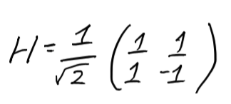
In order to translate a qubit into a superposition state, you need to apply a special transformation to it - the Hadamard Gate. Another use of Hadamard's gate will return the qubit to one of the basic states. This is the Hadamard gate matrix and an example of its use:
H × | 0⟩ = H × (1 | 0⟩ + 0 | 1⟩) = 1 / sqr (2) | 0⟩ + 1 / sqr (2) | 1⟩
H × (1 / sqr (2) | 0⟩ + 1 / sqr (2) | 1⟩) = 1 | 0⟩ + 0 | 1⟩ = | 0⟩
The action of the CNOT two-qubit gate with a controlling qubit in superposition is interesting: the CNOT confuses qubits. The entangled state is a phenomenon in which qubits cannot be considered separately, since their state is now common.
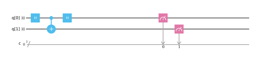
Let's give an example. Suppose we have a register of two qubits in the initial state — in the basic state | 0⟩). Apply Hadamard's gate to the first qubit - we get the following register state:
H × I × | 00⟩ = H × (1 | 0⟩ + 0 | 1⟩) × I × (1 | 0⟩ + 0 | 1⟩) = (1 / sqr (2) | 0⟩ + 1 / sqr (2) | 1⟩) × (1 | 0⟩ + 0 | 1⟩) =
1 / sqr (2) | 00⟩ + 1 / sqr (2) | 10⟩
The first and second qubits in this register are independent of each other. The second qubit is still in the state | 0⟩ and if we measure it, we still will not get information on the state of the first one - it can be either in the state 0 or in state 1. We use the two-qubit gate CNOT:
CNot × (1 / sqr (2) | 00⟩ + 1 / sqr (2) | 10⟩) = CNot × (1 / sqr (2) | 00⟩ + 0 | 01⟩ + 1 / sqr (2) | 10 ⟩ + 0 | 11⟩) =
1 / sqr (2) | 00⟩ + 0 | 01⟩ + 0 | 10⟩ + 1 / sqr (2) | 11⟩ = 1 / sqr (2) | 00⟩ + 1 / sqr (2) | 11⟩
Now the qubits are in a confused state, and the measurement of any of them will immediately cause the other to collapse! The state of the register shows that both qubits are in the same state - 0 or 1. So by measuring one, we will know exactly the state of the other.
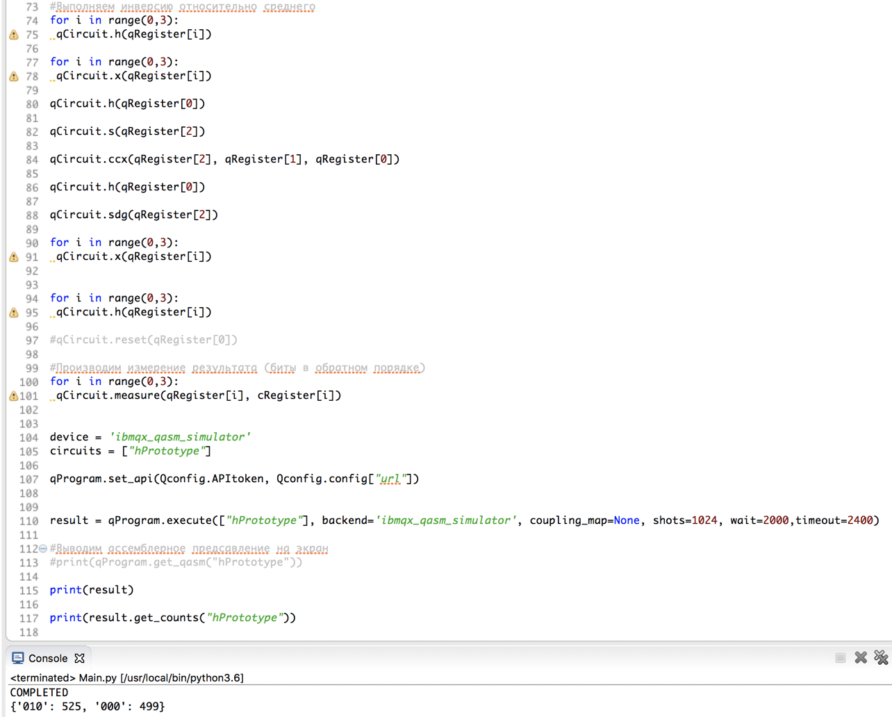
After we have confused the qubits, it is impossible to just collapse one of them into a basic state - they must first be unraveled. Try creating this scheme yourself using IBM's quantum editor and evaluate the result:
Making calculations on a quantum register of n qubits, we have the ability to simultaneously process all 2 n possible states. However, when measuring, each qubit collapses into one of its basic states, which means that after measuring the result, we have no opportunity to get more information than in the classical case - we only get one of the possible states with the corresponding probability.
Quantum algorithms take into account this property and offer many approaches to solve a particular class of problems. For example, in one of the approaches there are many such transformations that increase the amplitude of the desired solution and reduce the amplitudes of the others.
The algorithm representing the set of such transformations is called the Grover algorithm. It allows quadratically speed up searches in unstructured databases. Usually, the complexity of the search in an unstructured data set is O (n), that is, in the worst case, we need to look through all the records. The quantum algorithm allows solving this problem in O (√n).
For example, we have 40 bits and we need to find one of all possible combinations that satisfies some condition. In the classic case, we will need to process about 1,000,000,000,000 different combinations. The quantum algorithm will allow to get the result for 1,000,000.
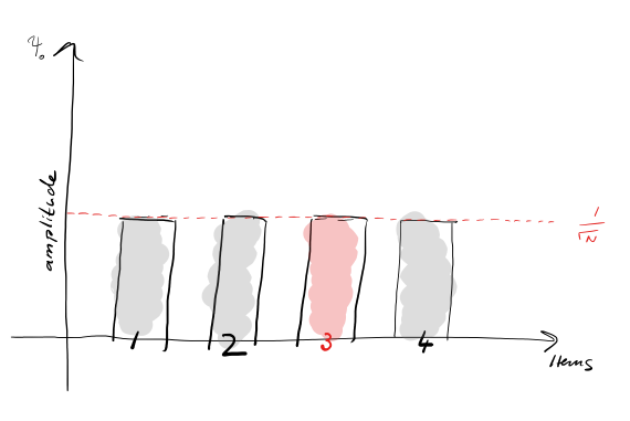
Consider an example. We have a register of n qubits in superposition. Thus, we have 2 n of all possible states, and the amplitude of each is 1 / √ 2 n (with this value the sum of the squares of the modules will be 1). Imagine this in the form of a diagram:
We also have one extra qubit, which we will call functional, and an oracle function. The Oracle translates the functional qubit from the base state | 0⟩ to the state | 1⟩ exactly on the set we are looking for.
In order to get exactly the state that corresponds to the oracle function during the measurement, we perform the following actions:
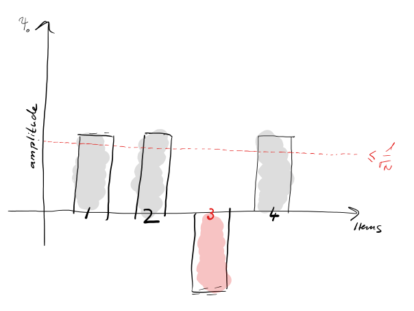 The dashed line in the figures indicates the average amplitude. After the sign of the target amplitude has changed, the average has fallen below.
Imagine, for example, that we need to find a number in the range from 0 to 7, which after a cyclic bit shift to the left will give a number less than 2. On a classical calculator, this class of problems is solved only by brute force. We would need to calculate our function (bit shift) on all arguments and then apply a condition to each result. The quantum algorithm allows you to do this instantly.
All the algorithms and techniques discussed earlier are valid for the so-called universal quantum computer - a computer capable of performing elementary transformations and actually solving any problem (in the simplest case, simulating a classical algorithm).
But there is a whole layer of mathematical problems in which, as such, calculations are not required, but it is necessary to find a combination of arguments in which a certain type of function will take the minimum value. This class of tasks — optimization problems — will be discussed in more detail below.
Annealing is a process of gradual cooling of a substance, in which the molecules gather against the background of slowing down of thermal motion in the most energetically favorable configurations. The term "annealing" came from metallurgy. In a more energetically favorable state, the metal becomes both harder and stronger: more external action is required, more mechanical work on the piece of metal to break the advantageous configuration of molecules, to “lift” this configuration over the very bottom of the energy well.
Like classical annealing, when the interparticle interaction is slowly turned on, the quantum system “looks for” the energetically most favorable configuration through the effects of quantum mechanics. Quantum computing based on quantum annealing can solve certain problems that are difficult to solve using classic computers.
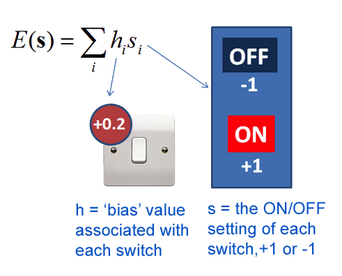
Consider a math problem known as “playing with light switches”. Its goal is to find the best on and off configurations for a variety of switches. Here is how it looks graphically:
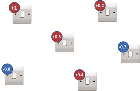
Imagine that each switch has a weight that we cannot change. We can enable (ON) or disable (OFF) each switch. ON stands for multiplication by 1, and OFF for -1. Then we add all the switch weights multiplied by their ON / OFF values. The goal of the game is to set the switches to get the lowest amount. The weight of the i-th switch is denoted by h i , and the switch state by s i .
Depending on which switches are set to ON or OFF, we get different totals. Finding the minimum amount will be easy, because there is a simple rule for the guaranteed minimum:
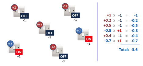
If we set all switches with positive indicators to the OFF position, and all switches with negative indicators - to the ON position, then in total we get the lowest total value.
Now let's complicate the task: add a new weight J. It will change in accordance with the ON / OFF states of adjacent switches. And then it is included in the total amount we received earlier.
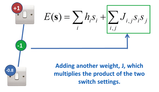
It is much more difficult now to decide whether the switch should be on or off because its neighbors influence it. Even in a simple example with two switches, we cannot simply set the ON / OFF parameter to the position opposite to the sign of the body weight of the switches. With a complex network of switches, the task becomes practically unsolvable.
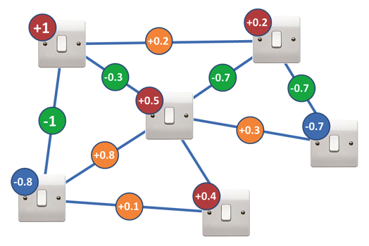
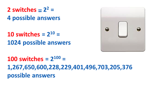
With a few switches, we can simply try each combination ON and OFF; there are only four possibilities: [ON ON], [ON OFF], [OFF ON] or [OFF OFF]. But as we add more and more switches, the number of possible ways to install switches increases exponentially:
How will quantum mechanics help? We start with the system in its quantum superposition, then use the quantum computer (DWave), which, using quantum optimization, finds for the switches the state in which the sum value will be the lowest.
Let's formulate a test problem and try to solve it using the DWave quantum computer. The task sounds like this - the bank has a collection service and a lot of ATMs in the city, from where you need to take money. The shorter the route, the less chance of getting into an unpleasant situation. Accordingly, we need to find the optimal route in a weighted directed graph with N vertices. This task is better known as the “Traveling Salesman Task” and does not have a better solution than full brute force.
In order to solve this problem, you must first understand how to solve problems on DWave. First we need to develop an input configuration file. It has the following format:
c
c This is a sample .qubo file
c with 4 nodes and 6 couplers
c
p qubo 0 4 4 6
c - 0 0 3.4
1 1 4.5
2 2 2.1
3 3 -2.4
c - 0 1 2.2
0 2 3.4
1 2 4.5
0 3 -2
0 2 3.4
1 2 4.5
0 3 -2
1 3 4.5678
2 3 -3.22
The lines with comments are marked with “c”, then we set the program parameters in the line beginning with the “p” character. In this line, we define the topology (so far it is always 0), the number of qubits (in terms of playing with light, these are “switches”) and the connections between pairs (“J” scales). Next is a block with a description of the weights of each qubit. In this block, the first two numbers must be the same, and they correspond to the qubit number. The next block is a block of link weights between pairs. The number of the first qubit should always be less than the second.
So, having understood the format, let's proceed to the solution of our problem.
First, we highlight the concept of a step of a path — this is the set of all possible vertices of the graph in which we can be at the current time. Each vertex is represented by a qubit. And we will have N such steps, where N is the number of vertices in our graph.
Suppose we have only 4 vertices, at each step we can be in one of 4 vertices, respectively, the entire set of qubits is divided into blocks of 4 qubits. In our case, from 4 vertices, we will need a register of 16 qubits, we number them - a 0 ... a 16 . Accordingly, in the first block there will be qubits with numbers a 0 ..a 3 - they correspond to being in one of the vertices in the first step.
Now we need to place the weights of the qubits and their connections inside one block so that only one qubit in each block in the final solution is in state 1, and the others in 0. This is due to the fact that in the end we can only be in one of vertices at every step. It is quite simple to do this - we set the weight of each qubit to -1, and the connections between them to 2. Indeed, if we look at the formula Σh i s i + ΣJ ij s i s j , then we will see that it will be minimal if the second The term will be zero. And this will happen only in two cases - if all qubits are equal to 0 or if one of them is in 1 and the others in 0. But at the same time, the first term will give a minimum in the second case.
So, we expose in this way the weights at all steps (blocks from the peaks) of our path. Now, if we send our program for execution, we will receive a response of the form (0001 0100 1000 1000). For convenience, we have divided them into blocks of 4 quits by spaces. We see that in each block there is only one unit, and its number in the block corresponds to the number of the vertex. In our solution there are blocks with the same number of vertices - 1000. We need to exclude such solutions, since we cannot return to the already completed peaks. In order to do this, we will consider new blocks - combining the same vertex at different steps.
Consider the block a 0 , a 4 , a 8 , a 12 . These qubits correspond to being in the first vertex at the corresponding step. Similar to the previous paragraph, only one of them must be equal to one - then we will be in the first vertex only once for the entire path. We set the link weights for all such blocks and send the program for execution. We receive the answer of a type (0001 0100 1000 0001 0010). Well, we have already got a path that matches the definition, now we need to find the optimal path according to the weights of the edges of the graph. To do this, we take the values from the adjacency matrix of the graph and transfer these values to our configuration. After that we get the result.
Solution before parsing
Solution after parsing
In fact, programming on a DWave quantum computer is a bit more complicated, since it is necessary to take into account the physical partition of the entire register into blocks of 8 qubits, etc. Without this, some of the combinations may not be considered, and as a result we will get some local minimum instead of a global one, but even such a simple program gives excellent results compared to classical methods.
We conducted a test run on 14 vertices on a specific graph. The search algorithm found the shortest path with a length of 91, the work took about 10 minutes. The Little method worked almost instantly and gave the result 104. The quantum algorithm also worked almost instantly and gave the result 97. At the same time, if the program on a quantum computer is built taking into account the physical connections, then we will get a result similar to the search.
The maximum graph, which at the moment we can process using a quantum calculator, contains 44 vertices. On a classical calculator, in general, it will take a disproportionately longer amount of time, since complexity grows by the formula n! ..
A quantum computer built on the principles of annealing, has more power than the existing universal computers, but it is limited to the class of tasks. We do not have the opportunity to set the initial states of the qubits or to perform any unitary transformations on them - we have only one possibility - to find a combination in which the value of the function Σh i s i + ΣJ ij s i s j with a given configuration will be minimal. However, even with this limitation, quantum computers show significant performance gains and can be effectively used in optimization problems.
At the moment there are the following main areas of implementation of quantum computers:
The most developed to date are the quantum computers DWave and IBM Q
DWave has the status of an “analog quantum computer”, as it is capable of solving only a narrow circle of quantum annealing problems. But at the same time, its declared capacity is 2,000 qubits.

IBM Q is a program for developing universal quantum computers on which arbitrary quantum algorithms can be executed. Currently, there are 20 qubit systems in operation (commercial use), and Q Experience open systems for 16 and 5 qubits. Q Experience now, perhaps, the only open platform that allows you to develop quantum algorithms. It is a set of atomic gates that can be applied to qubits.
In addition to the scenarios described earlier, quantum computing may work fine in other areas.
Quantum cryptography. Information security is based on the fact that the decryption task is not solvable. Quantum cryptography is based on the impossibility of breaking the laws of physics. One example is the exchange of BB84 secret keys. Vasya gives Masha a set of quantum particles. Jealous attacker Petya listens on the communication channel and can intercept particles. But for this Petya will have to measure them. He will inevitably destroy their original state, which Vasya and Masha will know.
Blockchain protection. In principle, it is based on the fact that miners need a large amount of time in order to use the search to find the number at which the block hash is less than a certain threshold. This does not allow to replace the block - until the new hash is calculated, the chain will go far ahead. Due to parallelism, a quantum blockchain can instantly find a number at which the block hash will be unattainably small for classical computers. Thus, it will be possible to attack the network only if 51% of quantum miners are captured. And this brings trust to a new level - collusion of more than half of players with such opportunities is unlikely.
It is known that in 2014, Chinese researchers first implemented handwriting recognition using quantum computing.
Finally, instant processing of a colossal amount of data and solving optimization problems make quantum technologies one of the most promising tools in the field of artificial intelligence and machine learning. For this reason, in 2013, Google and NASA created a joint research laboratory in this area.
Based on the materials of Dmitry Sapaev , senior director of IT systems development in the development department of Sberbank Technologies TIC, and Dmitry Bulychkov, project director at the Center for Technological Innovations of Sberbank.
Quantum parallelism
According to the laws of quantum mechanics, a particle can be in all its states at the same time. This qubit state is called superposition. In the superposition, the amplitudes of the basis states take nonzero values - a | 0⟩ + b | 1⟩ and the normalization requirement is preserved.
A quantum particle can be in superposition only until the moment of measurement. After measurement, it collapses into one of its basic states, 0 or 1. If we have a register of qubits that are in superposition, then the state of the register itself can be defined as follows:
')
(a 0 | 0⟩ + b 0 | 1⟩) (a 1 | 0⟩ + b 1 | 1⟩) ... (a n | 0⟩ + b n | 1⟩) =
a 0 × a 1 ×… × a n | 00..0⟩ + a 0 × a 1 × ... × b n | 00 ... 1⟩ + ... + b 0 × b 1 × ... × b n | 11 ... 1⟩
It is important to understand that the factors that face states are not a probability. Otherwise, we would get a classical system with a restriction — it is not known what state it is in. And the quantum bit is in both states at the same time. We have the ability to process all 2 n possible combinations at once!
In order to translate a qubit into a superposition state, you need to apply a special transformation to it - the Hadamard Gate. Another use of Hadamard's gate will return the qubit to one of the basic states. This is the Hadamard gate matrix and an example of its use:
H × | 0⟩ = H × (1 | 0⟩ + 0 | 1⟩) = 1 / sqr (2) | 0⟩ + 1 / sqr (2) | 1⟩
H × (1 / sqr (2) | 0⟩ + 1 / sqr (2) | 1⟩) = 1 | 0⟩ + 0 | 1⟩ = | 0⟩
The action of the CNOT two-qubit gate with a controlling qubit in superposition is interesting: the CNOT confuses qubits. The entangled state is a phenomenon in which qubits cannot be considered separately, since their state is now common.
Let's give an example. Suppose we have a register of two qubits in the initial state — in the basic state | 0⟩). Apply Hadamard's gate to the first qubit - we get the following register state:
H × I × | 00⟩ = H × (1 | 0⟩ + 0 | 1⟩) × I × (1 | 0⟩ + 0 | 1⟩) = (1 / sqr (2) | 0⟩ + 1 / sqr (2) | 1⟩) × (1 | 0⟩ + 0 | 1⟩) =
1 / sqr (2) | 00⟩ + 1 / sqr (2) | 10⟩
The first and second qubits in this register are independent of each other. The second qubit is still in the state | 0⟩ and if we measure it, we still will not get information on the state of the first one - it can be either in the state 0 or in state 1. We use the two-qubit gate CNOT:
CNot × (1 / sqr (2) | 00⟩ + 1 / sqr (2) | 10⟩) = CNot × (1 / sqr (2) | 00⟩ + 0 | 01⟩ + 1 / sqr (2) | 10 ⟩ + 0 | 11⟩) =
1 / sqr (2) | 00⟩ + 0 | 01⟩ + 0 | 10⟩ + 1 / sqr (2) | 11⟩ = 1 / sqr (2) | 00⟩ + 1 / sqr (2) | 11⟩
Now the qubits are in a confused state, and the measurement of any of them will immediately cause the other to collapse! The state of the register shows that both qubits are in the same state - 0 or 1. So by measuring one, we will know exactly the state of the other.
After we have confused the qubits, it is impossible to just collapse one of them into a basic state - they must first be unraveled. Try creating this scheme yourself using IBM's quantum editor and evaluate the result:
Collapse and the amount of information received
Making calculations on a quantum register of n qubits, we have the ability to simultaneously process all 2 n possible states. However, when measuring, each qubit collapses into one of its basic states, which means that after measuring the result, we have no opportunity to get more information than in the classical case - we only get one of the possible states with the corresponding probability.
Quantum algorithms take into account this property and offer many approaches to solve a particular class of problems. For example, in one of the approaches there are many such transformations that increase the amplitude of the desired solution and reduce the amplitudes of the others.
Grover's algorithm
The algorithm representing the set of such transformations is called the Grover algorithm. It allows quadratically speed up searches in unstructured databases. Usually, the complexity of the search in an unstructured data set is O (n), that is, in the worst case, we need to look through all the records. The quantum algorithm allows solving this problem in O (√n).
For example, we have 40 bits and we need to find one of all possible combinations that satisfies some condition. In the classic case, we will need to process about 1,000,000,000,000 different combinations. The quantum algorithm will allow to get the result for 1,000,000.
Consider an example. We have a register of n qubits in superposition. Thus, we have 2 n of all possible states, and the amplitude of each is 1 / √ 2 n (with this value the sum of the squares of the modules will be 1). Imagine this in the form of a diagram:
We also have one extra qubit, which we will call functional, and an oracle function. The Oracle translates the functional qubit from the base state | 0⟩ to the state | 1⟩ exactly on the set we are looking for.
In order to get exactly the state that corresponds to the oracle function during the measurement, we perform the following actions:
- Change the amplitude of the desired value to negative. To do this, we translate the functional qubit to the state | 1⟩ on all sets, then apply the Hadamard gate to it and then the oracle function to the entire register. After this action, the picture will look like this:
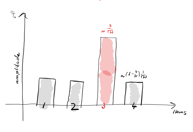
- Since we process all states in the same way, we cannot change any one amplitude. But we can make an inversion with respect to the mean — display the amplitude value, taking the mean value by the axis:
- As we can see, the value of the desired amplitude has grown relative to the rest. According to the results of performing this set of actions of order Pi × 0.25 × √2 n times, the sought amplitude will be almost equal to one.
Imagine, for example, that we need to find a number in the range from 0 to 7, which after a cyclic bit shift to the left will give a number less than 2. On a classical calculator, this class of problems is solved only by brute force. We would need to calculate our function (bit shift) on all arguments and then apply a condition to each result. The quantum algorithm allows you to do this instantly.
Quantum optimization
All the algorithms and techniques discussed earlier are valid for the so-called universal quantum computer - a computer capable of performing elementary transformations and actually solving any problem (in the simplest case, simulating a classical algorithm).
But there is a whole layer of mathematical problems in which, as such, calculations are not required, but it is necessary to find a combination of arguments in which a certain type of function will take the minimum value. This class of tasks — optimization problems — will be discussed in more detail below.
Quantum annealing
Annealing is a process of gradual cooling of a substance, in which the molecules gather against the background of slowing down of thermal motion in the most energetically favorable configurations. The term "annealing" came from metallurgy. In a more energetically favorable state, the metal becomes both harder and stronger: more external action is required, more mechanical work on the piece of metal to break the advantageous configuration of molecules, to “lift” this configuration over the very bottom of the energy well.
Like classical annealing, when the interparticle interaction is slowly turned on, the quantum system “looks for” the energetically most favorable configuration through the effects of quantum mechanics. Quantum computing based on quantum annealing can solve certain problems that are difficult to solve using classic computers.
Consider a math problem known as “playing with light switches”. Its goal is to find the best on and off configurations for a variety of switches. Here is how it looks graphically:
Imagine that each switch has a weight that we cannot change. We can enable (ON) or disable (OFF) each switch. ON stands for multiplication by 1, and OFF for -1. Then we add all the switch weights multiplied by their ON / OFF values. The goal of the game is to set the switches to get the lowest amount. The weight of the i-th switch is denoted by h i , and the switch state by s i .
Depending on which switches are set to ON or OFF, we get different totals. Finding the minimum amount will be easy, because there is a simple rule for the guaranteed minimum:
If we set all switches with positive indicators to the OFF position, and all switches with negative indicators - to the ON position, then in total we get the lowest total value.
Now let's complicate the task: add a new weight J. It will change in accordance with the ON / OFF states of adjacent switches. And then it is included in the total amount we received earlier.
It is much more difficult now to decide whether the switch should be on or off because its neighbors influence it. Even in a simple example with two switches, we cannot simply set the ON / OFF parameter to the position opposite to the sign of the body weight of the switches. With a complex network of switches, the task becomes practically unsolvable.
With a few switches, we can simply try each combination ON and OFF; there are only four possibilities: [ON ON], [ON OFF], [OFF ON] or [OFF OFF]. But as we add more and more switches, the number of possible ways to install switches increases exponentially:
How will quantum mechanics help? We start with the system in its quantum superposition, then use the quantum computer (DWave), which, using quantum optimization, finds for the switches the state in which the sum value will be the lowest.
"The task of the collector"
Let's formulate a test problem and try to solve it using the DWave quantum computer. The task sounds like this - the bank has a collection service and a lot of ATMs in the city, from where you need to take money. The shorter the route, the less chance of getting into an unpleasant situation. Accordingly, we need to find the optimal route in a weighted directed graph with N vertices. This task is better known as the “Traveling Salesman Task” and does not have a better solution than full brute force.
In order to solve this problem, you must first understand how to solve problems on DWave. First we need to develop an input configuration file. It has the following format:
c
c This is a sample .qubo file
c with 4 nodes and 6 couplers
c
p qubo 0 4 4 6
c - 0 0 3.4
1 1 4.5
2 2 2.1
3 3 -2.4
c - 0 1 2.2
0 2 3.4
1 2 4.5
0 3 -2
0 2 3.4
1 2 4.5
0 3 -2
1 3 4.5678
2 3 -3.22
The lines with comments are marked with “c”, then we set the program parameters in the line beginning with the “p” character. In this line, we define the topology (so far it is always 0), the number of qubits (in terms of playing with light, these are “switches”) and the connections between pairs (“J” scales). Next is a block with a description of the weights of each qubit. In this block, the first two numbers must be the same, and they correspond to the qubit number. The next block is a block of link weights between pairs. The number of the first qubit should always be less than the second.
So, having understood the format, let's proceed to the solution of our problem.
First, we highlight the concept of a step of a path — this is the set of all possible vertices of the graph in which we can be at the current time. Each vertex is represented by a qubit. And we will have N such steps, where N is the number of vertices in our graph.
Suppose we have only 4 vertices, at each step we can be in one of 4 vertices, respectively, the entire set of qubits is divided into blocks of 4 qubits. In our case, from 4 vertices, we will need a register of 16 qubits, we number them - a 0 ... a 16 . Accordingly, in the first block there will be qubits with numbers a 0 ..a 3 - they correspond to being in one of the vertices in the first step.
Now we need to place the weights of the qubits and their connections inside one block so that only one qubit in each block in the final solution is in state 1, and the others in 0. This is due to the fact that in the end we can only be in one of vertices at every step. It is quite simple to do this - we set the weight of each qubit to -1, and the connections between them to 2. Indeed, if we look at the formula Σh i s i + ΣJ ij s i s j , then we will see that it will be minimal if the second The term will be zero. And this will happen only in two cases - if all qubits are equal to 0 or if one of them is in 1 and the others in 0. But at the same time, the first term will give a minimum in the second case.
So, we expose in this way the weights at all steps (blocks from the peaks) of our path. Now, if we send our program for execution, we will receive a response of the form (0001 0100 1000 1000). For convenience, we have divided them into blocks of 4 quits by spaces. We see that in each block there is only one unit, and its number in the block corresponds to the number of the vertex. In our solution there are blocks with the same number of vertices - 1000. We need to exclude such solutions, since we cannot return to the already completed peaks. In order to do this, we will consider new blocks - combining the same vertex at different steps.
Consider the block a 0 , a 4 , a 8 , a 12 . These qubits correspond to being in the first vertex at the corresponding step. Similar to the previous paragraph, only one of them must be equal to one - then we will be in the first vertex only once for the entire path. We set the link weights for all such blocks and send the program for execution. We receive the answer of a type (0001 0100 1000 0001 0010). Well, we have already got a path that matches the definition, now we need to find the optimal path according to the weights of the edges of the graph. To do this, we take the values from the adjacency matrix of the graph and transfer these values to our configuration. After that we get the result.
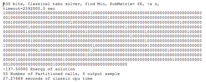
Solution before parsing
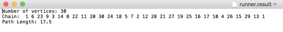
Solution after parsing
In fact, programming on a DWave quantum computer is a bit more complicated, since it is necessary to take into account the physical partition of the entire register into blocks of 8 qubits, etc. Without this, some of the combinations may not be considered, and as a result we will get some local minimum instead of a global one, but even such a simple program gives excellent results compared to classical methods.
We conducted a test run on 14 vertices on a specific graph. The search algorithm found the shortest path with a length of 91, the work took about 10 minutes. The Little method worked almost instantly and gave the result 104. The quantum algorithm also worked almost instantly and gave the result 97. At the same time, if the program on a quantum computer is built taking into account the physical connections, then we will get a result similar to the search.
The maximum graph, which at the moment we can process using a quantum calculator, contains 44 vertices. On a classical calculator, in general, it will take a disproportionately longer amount of time, since complexity grows by the formula n! ..
A quantum computer built on the principles of annealing, has more power than the existing universal computers, but it is limited to the class of tasks. We do not have the opportunity to set the initial states of the qubits or to perform any unitary transformations on them - we have only one possibility - to find a combination in which the value of the function Σh i s i + ΣJ ij s i s j with a given configuration will be minimal. However, even with this limitation, quantum computers show significant performance gains and can be effectively used in optimization problems.
Quantum computers today
At the moment there are the following main areas of implementation of quantum computers:
- On ions in a one-dimensional ionic crystal trapped in Paul.
- In semiconductor crystals of a spinless monoisotopic silicon crystal
- Qubits on electrons in semiconductor quantum dots.
- Qubits on superconducting mesostructures.
- On single atoms in microresonators.
- With the help of linear optical elements (optical quantum computer).
The most developed to date are the quantum computers DWave and IBM Q
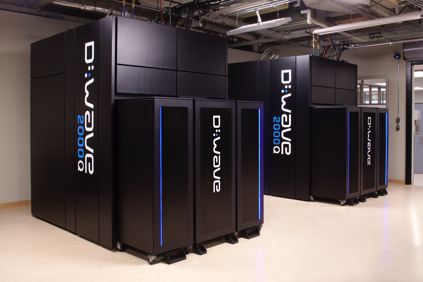
DWave has the status of an “analog quantum computer”, as it is capable of solving only a narrow circle of quantum annealing problems. But at the same time, its declared capacity is 2,000 qubits.
IBM Q is a program for developing universal quantum computers on which arbitrary quantum algorithms can be executed. Currently, there are 20 qubit systems in operation (commercial use), and Q Experience open systems for 16 and 5 qubits. Q Experience now, perhaps, the only open platform that allows you to develop quantum algorithms. It is a set of atomic gates that can be applied to qubits.
Using quantum computing
In addition to the scenarios described earlier, quantum computing may work fine in other areas.
Quantum cryptography. Information security is based on the fact that the decryption task is not solvable. Quantum cryptography is based on the impossibility of breaking the laws of physics. One example is the exchange of BB84 secret keys. Vasya gives Masha a set of quantum particles. Jealous attacker Petya listens on the communication channel and can intercept particles. But for this Petya will have to measure them. He will inevitably destroy their original state, which Vasya and Masha will know.
Blockchain protection. In principle, it is based on the fact that miners need a large amount of time in order to use the search to find the number at which the block hash is less than a certain threshold. This does not allow to replace the block - until the new hash is calculated, the chain will go far ahead. Due to parallelism, a quantum blockchain can instantly find a number at which the block hash will be unattainably small for classical computers. Thus, it will be possible to attack the network only if 51% of quantum miners are captured. And this brings trust to a new level - collusion of more than half of players with such opportunities is unlikely.
It is known that in 2014, Chinese researchers first implemented handwriting recognition using quantum computing.
Finally, instant processing of a colossal amount of data and solving optimization problems make quantum technologies one of the most promising tools in the field of artificial intelligence and machine learning. For this reason, in 2013, Google and NASA created a joint research laboratory in this area.
Based on the materials of Dmitry Sapaev , senior director of IT systems development in the development department of Sberbank Technologies TIC, and Dmitry Bulychkov, project director at the Center for Technological Innovations of Sberbank.
Source: https://habr.com/ru/post/344830/
All Articles