Deep Learning with Spark and Hadoop: Meet Deeplearning4j
Hello, dear readers!
We are fully convinced of the mega-popularity of deep learning (Python) in our target audience. Now we offer to talk about the major league of deep learning - that is, about solving these problems in the Java language with the help of the Deeplearning4j library. We have translated for you the June article from the Cloudera company blog, where the most interesting details are about the specifics of this library and about the deep learning in Hadoop and Spark.
Enjoy reading.
At the end of 2016, Ben Lorica from O'Reilly Media announced that “in 2017, the data science and big data community will be seriously engaged in AI technologies.” Until 2017, mostly deep GPU education was practiced at universities and research institutes , but at the present time, distributed, deep learning is spreading on the CPU in different companies and subject areas. While GPUs provide maximum performance in numerical calculations, modern CPUs also pull up to them in terms of efficiency, both due to improved equipment and for the reason that they can now be used "en masse". Such free tools have appeared, the most interesting of which is the deeplearning4j library - they provide fast deep learning in large-scale systems (the Hadoop stack) and should generally have a significant impact on deep learning in the coming years.
')
In this article, we take a closer look at working with free tools - Apache Spark, Apache Hadoop, Deeplearning4j (DL4J) - running on low-cost (and widely available) hardware. We will try to solve the problem of pattern recognition as efficiently as possible with a limited set of training data. The DL4J API library is written in Java and is particularly interesting to Java and Scala developers who already know how to use the Java virtual machine. In addition, the ability to parallelize model training in Spark (this requires only a few lines of code) simplifies the efficient use of existing cluster resources. Thus, the learning process can be accelerated without sacrificing accuracy.
Deeplearning4j: a tool for deep learning on JVM
Deeplearning4j is one of the many free kits for large-scale learning of deep neural networks on the CPU and GPU. Deeplearning4j is designed for the JVM and is specifically focused on deep learning for large enterprises. The deeplearning4j library was created in 2014, supported by Skymind startup and has built-in integration with Apache Spark. Although deeplearning4j is designed to work with JVM, it uses the high-performance native library of linear algebra Nd4j, which allows you to perform highly optimized calculations on a CPU or GPU.
Classification of objects from the set of images Caltech-256
This article explains how to use Apache Spark, Apache Hadoop and deeplearning4j to solve the problem of image classification. In particular, it describes step by step how to build a convolutional neural network capable of classifying images from the Caltech-256 set . In fact, there are 257 categories of objects in this set, each of which contains from 80 to 800 images; Thus, in total in this set we have 30,607 images.
It should be noted that the maximum classification accuracy of this data set currently ranges from 72 to 75%. This result can be beaten with DL4J and Spark.
Effective deep learning on small data
Modern convolutional networks can have several hundreds of millions of parameters. One of the most powerful of these networks is called the Large Scale Visual Recognition Challenge (also known as “ImageNet”), you need to train 140 million parameters in it! Such networks not only consume a lot of computing and disk resources (even if there is a cluster of GPUs, it can take weeks to train), but they also require a lot of data. With only 30,000 images, it is impractical to train such a complex model on Caltech-256, since there are too few examples in this set to adequately train so many parameters. It is better to use a method called “ learning transfer ”, in which a pre-trained model is taken, adapted for other use cases. Transfer of training also allows you to significantly reduce the computational load and get rid of numerous specialized computing resources, for example, the GPU.
Such models can be reoriented, since convolutional neural networks trained on sets of images usually isolate the most common features , and it is this kind of training based on features that can be useful when processing other sets of images. For example, a network trained on ImageNet will most likely recognize shapes, facial features, patterns, text, etc., which will undoubtedly come in handy when processing a Caltech-256 dataset.
Download pre-trained model
The following example uses the VGG16 model, which ranked second in the 2014 ImageNet competition. Fortunately, now this model is shared, all 140 million scales have already been optimized for forecasting on the ImageNet set. Since we are going to work with a different set of images, it will be necessary to modify small elements of the model in order to sharpen it for such a prediction. This model has about 140 million parameters, occupies about 500 MB of disk space.
To begin with, we will get such a version of the VGG16 model, which is understandable by DL4J, and with which this library can work. It turns out that this feature is built right into the DL4J API and is implemented in just a few lines on Scala.
Now our model is in a format that is convenient to use in DL4J. We investigate the built-in model summary.
Here is a beautiful and concise general description of the model; however, it is very useful to show it in the form of a picture.
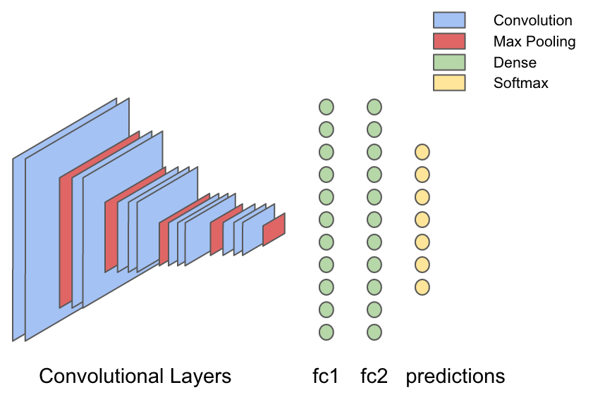
In VGG16, there are 13 convolutional layers interspersed with layers in which the maximum value is selected (max-pooling); This is done to compress the image. Weight values in the convolutional layer are, in essence, filters that learn to isolate visual features from the image, and layers with the choice of the maximum value “compress” the image — and therefore the filters in the next convolutional layers will “see” the image more fully. Therefore, the result of the work of convolutional layers is the most common visual signs of the input image, for example, “is there a face in the picture?” Or “a sunset in the picture?”. The result of the work of convolutional layers is supplied to a series of three fully connected (dense) layers capable of learning the nonlinear interconnections between these visual characteristics and output information.
This is one of the main properties of convolutional networks, which ensures the transfer of learning. The point is that you can skip the new information about the images through the already trained VGG16 network and isolate the signs from each image. Such an operation is called “characterization” (featurizing): after extracting the signs, it remains to work only with the last parts of the VGG16 network, and this task is much more advanced both from a computational point of view and in terms of complexity.
Characterization of images with VGG16
The data set can be downloaded from the Caltech-256 site, where it is divided into fragments for training / checking / testing and stored in HDFS ( detailed instructions ). When this is done, we take the entire set of images and pass it through all the convolutional layers, as well as through the first dense layer, and save the output in HDFS.
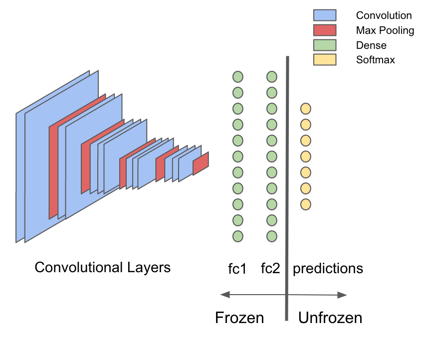
For some reason, it is desirable to do this and, to understand the importance of this approach, we note one general rule regarding convolution networks: most of the computer time and computational power is spent in convolutional layers, and most of the parameters (weights) in the VGG16 network are localized in dense layers. Due to the transfer of training, you can use pre-trained convolutional layers to extract features of the input images, so you have to retrain only a small part of the original model - dense layers. The rest remains static or "frozen." You can save a lot of time and computing power by transferring the raw images only once through the frozen part of the network, and then not returning to this part at all.
First we extract the part of the network that will be used at the characterization stage. The deeplearning4j library has a built-in API for transferring training, which can be used for this purpose. To separate the model after the first fully connected layer “fc1”, we first obtain a list of layers before and after separation.
Now we take the org.deeplearning4j.nn.transferlearning package to extract only layers up to "fc2" inclusive.
Next, you need to go to actually read image files, which are stored in HDFS in JPEG format, each separately. Images are arranged in subdirectories, and each subdirectory contains a set of pictures belonging to a particular class. Let's start uploading images saved in HDFS using sc.binaryFiles and use image processing tools from the DataVec library (native ETL library for DL4J) and using them to convert images into INDArray arrays, which are native tensor representations consumed by DL4J (full code here ). Finally, we use a frozen graph to issue predictions for input images: in essence, we pass them through expensive layers that will be discarded.
Now the new data set is saved in HDFS, and with its help you can start building models with the transfer of training. Such data with signs allows you to radically reduce the duration of training and reduce the complexity of calculations. In the above example, the new data consists of 30,607 vectors of 4096 length.
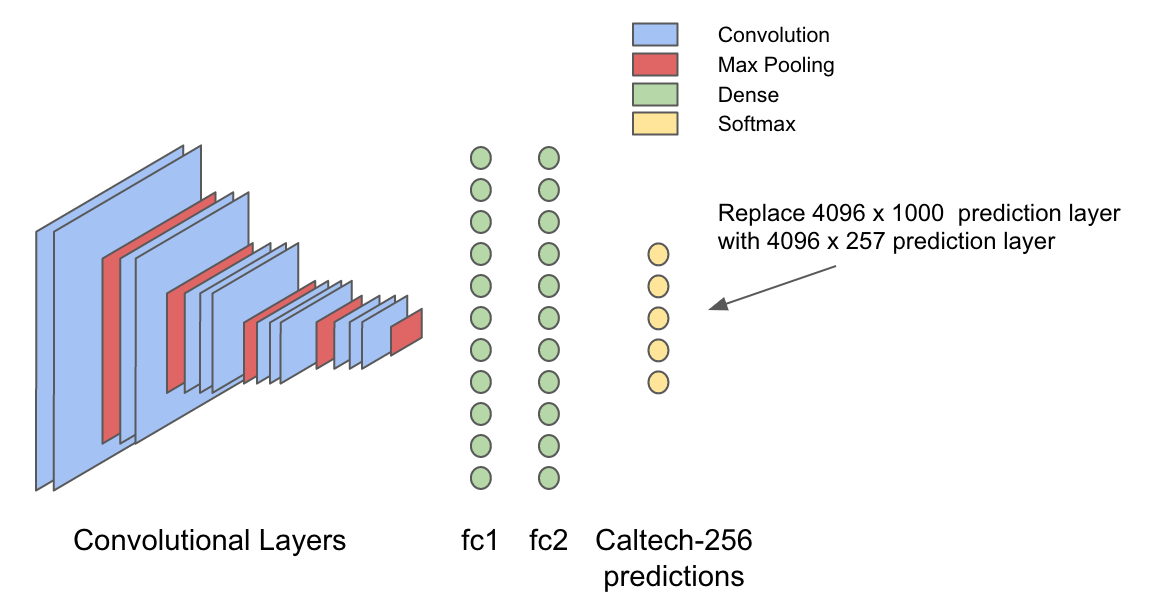
Replacing the VGG16 prediction layer
The VGG16 model was trained on the ImageNet dataset, which is a set of classified objects, divided into 1000 different categories. The last layer in a typical neural network to classify images, the so-called "output layer", on the basis of the input generates probabilities for each object contained in the data set. Therefore, such input can be considered as a generalized picture of the visual features of an image containing useful information about what an object is and what it contains. It is intuitively clear that the same “generalized” input entering the last layer should also be useful for generating a different set of probabilities, optimized for recognizing objects in the Caltech-256 data set.
After characterizing the data using the principle described above, we define a new model that occupies the 4096-dimensional inference in the fc2 layer and generates 257 probabilities for the Caltech256 data set.
Here's what it looks like.
So, now this model can be trained with the help of heavy calculations DL4J and scaled with Spark. For training in Spark, we use the
Now we teach
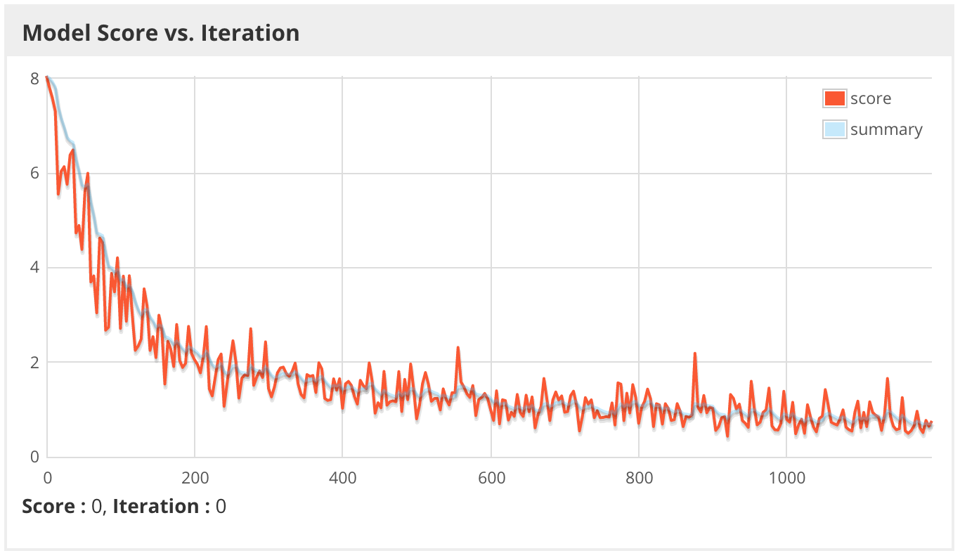
Finally, we start the training task with the help of spark submit and through the graphic web interface DL4J we monitor progress and diagnose problems. Below we see the “score” of the model — this indicator in this case means the negative log likelihood of the mini-block, the smaller the better. On the graph, it is depicted in relation to the "raw" values (numbers) and a smoothed trend line. Keep in mind that when training with Spark, the “account” of each mini-block actually corresponds to only one core in a Spark cluster, and we may have thousands of such cores. Ideally, the score on one core should match the count on the other, but if the data is not randomly randomized, then these indicators in the cluster can differ dramatically from core to core.
Apparently, this time, the model learns much faster, even with a lower coefficient of learning speed, since the signs used this time have a much higher predictive value than the ImageNet probabilities.
It seems that in this case the model has been retrained, since the learning accuracy is 88.8%, and the verification accuracy is only 76.3%. To make sure that the model does not retrain on the test set, we will evaluate it on a blind test set.
Although the accuracy has slightly decreased, it still surpasses the cutting-edge results for this data set, and in fact we used a simple architecture for deep learning, built on the basis of a ready-made Hadoop architecture and cheap CPUs! Yes, not a titanic achievement, however, this result still helps to test what can be achieved with the help of deep learning in Java.
findings
Although the deeplearning4j library is just one of many tools for deep learning, it is equipped with native integration with Apache Spark and written in Java, therefore it fits particularly well with the Hadoop ecosystem. Since access to information in enterprises is universally provided through Hadoop, and its processing takes place in Spark, the library deeplearning4j allows you to speed up the deployment and reduce costs, and you can immediately extract such information obtained by deep learning. The library uses ND4J for complex computations - another well-optimized library that interacts well with low-cost CPUs, but also supports GPU operations when it comes to dramatically increasing performance. Deeplearning4j is a full-featured library for deep learning, it has a complete set of tools to handle data from consumption to deployment. With this library, you can solve all sorts of tasks: image and video recognition, audio processing, natural language processing, creation of recommender systems, etc.
We are fully convinced of the mega-popularity of deep learning (Python) in our target audience. Now we offer to talk about the major league of deep learning - that is, about solving these problems in the Java language with the help of the Deeplearning4j library. We have translated for you the June article from the Cloudera company blog, where the most interesting details are about the specifics of this library and about the deep learning in Hadoop and Spark.
Enjoy reading.
At the end of 2016, Ben Lorica from O'Reilly Media announced that “in 2017, the data science and big data community will be seriously engaged in AI technologies.” Until 2017, mostly deep GPU education was practiced at universities and research institutes , but at the present time, distributed, deep learning is spreading on the CPU in different companies and subject areas. While GPUs provide maximum performance in numerical calculations, modern CPUs also pull up to them in terms of efficiency, both due to improved equipment and for the reason that they can now be used "en masse". Such free tools have appeared, the most interesting of which is the deeplearning4j library - they provide fast deep learning in large-scale systems (the Hadoop stack) and should generally have a significant impact on deep learning in the coming years.
')
In this article, we take a closer look at working with free tools - Apache Spark, Apache Hadoop, Deeplearning4j (DL4J) - running on low-cost (and widely available) hardware. We will try to solve the problem of pattern recognition as efficiently as possible with a limited set of training data. The DL4J API library is written in Java and is particularly interesting to Java and Scala developers who already know how to use the Java virtual machine. In addition, the ability to parallelize model training in Spark (this requires only a few lines of code) simplifies the efficient use of existing cluster resources. Thus, the learning process can be accelerated without sacrificing accuracy.
Deeplearning4j: a tool for deep learning on JVM
Deeplearning4j is one of the many free kits for large-scale learning of deep neural networks on the CPU and GPU. Deeplearning4j is designed for the JVM and is specifically focused on deep learning for large enterprises. The deeplearning4j library was created in 2014, supported by Skymind startup and has built-in integration with Apache Spark. Although deeplearning4j is designed to work with JVM, it uses the high-performance native library of linear algebra Nd4j, which allows you to perform highly optimized calculations on a CPU or GPU.
Classification of objects from the set of images Caltech-256
This article explains how to use Apache Spark, Apache Hadoop and deeplearning4j to solve the problem of image classification. In particular, it describes step by step how to build a convolutional neural network capable of classifying images from the Caltech-256 set . In fact, there are 257 categories of objects in this set, each of which contains from 80 to 800 images; Thus, in total in this set we have 30,607 images.
It should be noted that the maximum classification accuracy of this data set currently ranges from 72 to 75%. This result can be beaten with DL4J and Spark.
Effective deep learning on small data
Modern convolutional networks can have several hundreds of millions of parameters. One of the most powerful of these networks is called the Large Scale Visual Recognition Challenge (also known as “ImageNet”), you need to train 140 million parameters in it! Such networks not only consume a lot of computing and disk resources (even if there is a cluster of GPUs, it can take weeks to train), but they also require a lot of data. With only 30,000 images, it is impractical to train such a complex model on Caltech-256, since there are too few examples in this set to adequately train so many parameters. It is better to use a method called “ learning transfer ”, in which a pre-trained model is taken, adapted for other use cases. Transfer of training also allows you to significantly reduce the computational load and get rid of numerous specialized computing resources, for example, the GPU.
Such models can be reoriented, since convolutional neural networks trained on sets of images usually isolate the most common features , and it is this kind of training based on features that can be useful when processing other sets of images. For example, a network trained on ImageNet will most likely recognize shapes, facial features, patterns, text, etc., which will undoubtedly come in handy when processing a Caltech-256 dataset.
Download pre-trained model
The following example uses the VGG16 model, which ranked second in the 2014 ImageNet competition. Fortunately, now this model is shared, all 140 million scales have already been optimized for forecasting on the ImageNet set. Since we are going to work with a different set of images, it will be necessary to modify small elements of the model in order to sharpen it for such a prediction. This model has about 140 million parameters, occupies about 500 MB of disk space.
To begin with, we will get such a version of the VGG16 model, which is understandable by DL4J, and with which this library can work. It turns out that this feature is built right into the DL4J API and is implemented in just a few lines on Scala.
val modelImportHelper = new TrainedModelHelper(TrainedModels.VGG16) val vgg16 = modelImportHelper.loadModel() val savePath = "./dl4j-models/vgg16.zip" val locationToSave = new File(savePath) // DL4J, ModelSerializer.writeModel(vgg16, locationToSave, saveUpdater = true) Now our model is in a format that is convenient to use in DL4J. We investigate the built-in model summary.
val modelFile = new File("./dl4j-models/vgg16.zip") val vgg16 = ModelSerializer.restoreComputationGraph(modelFile) println(vgg16.summary()) VertexName (VertexType) nIn,nOut TotalParams ParamsShape Vertex Inputs input_2 (InputVertex) -,- - - - block1_conv1 (ConvolutionLayer) 3,64 1792 b:{1,64}, W:{64,3,3,3} [input_2] block1_conv2 (ConvolutionLayer) 64,64 36928 b:{1,64}, W:{64,64,3,3} [block1_conv1] block1_pool (SubsamplingLayer) -,- 0 - [block1_conv2] block2_conv1 (ConvolutionLayer) 64,128 73856 b:{1,128}, W:{128,64,3,3} [block1_pool] block2_conv2 (ConvolutionLayer) 128,128 147584 b:{1,128}, W:{128,128,3,3} [block2_conv1] block2_pool (SubsamplingLayer) -,- 0 - [block2_conv2] block3_conv1 (ConvolutionLayer) 128,256 295168 b:{1,256}, W:{256,128,3,3} [block2_pool] block3_conv2 (ConvolutionLayer) 256,256 590080 b:{1,256}, W:{256,256,3,3} [block3_conv1] block3_conv3 (ConvolutionLayer) 256,256 590080 b:{1,256}, W:{256,256,3,3} [block3_conv2] block3_pool (SubsamplingLayer) -,- 0 - [block3_conv3] block4_conv1 (ConvolutionLayer) 256,512 1180160 b:{1,512}, W:{512,256,3,3} [block3_pool] block4_conv2 (ConvolutionLayer) 512,512 2359808 b:{1,512}, W:{512,512,3,3} [block4_conv1] block4_conv3 (ConvolutionLayer) 512,512 2359808 b:{1,512}, W:{512,512,3,3} [block4_conv2] block4_pool (SubsamplingLayer) -,- 0 - [block4_conv3] block5_conv1 (ConvolutionLayer) 512,512 2359808 b:{1,512}, W:{512,512,3,3} [block4_pool] block5_conv2 (ConvolutionLayer) 512,512 2359808 b:{1,512}, W:{512,512,3,3} [block5_conv1] block5_conv3 (ConvolutionLayer) 512,512 2359808 b:{1,512}, W:{512,512,3,3} [block5_conv2] block5_pool (SubsamplingLayer) -,- 0 - [block5_conv3] flatten (PreprocessorVertex) -,- - - [block5_pool] fc1 (DenseLayer) 25088,4096 102764544 b:{1,4096}, W:{25088,4096} [flatten] fc2 (DenseLayer) 4096,4096 16781312 b:{1,4096}, W:{4096,4096} [fc1] predictions (DenseLayer) 4096,1000 4097000 b:{1,1000}, W:{4096,1000} [fc2] Total Parameters: 138357544 Trainable Parameters: 138357544 Frozen Parameters: 0 Here is a beautiful and concise general description of the model; however, it is very useful to show it in the form of a picture.
In VGG16, there are 13 convolutional layers interspersed with layers in which the maximum value is selected (max-pooling); This is done to compress the image. Weight values in the convolutional layer are, in essence, filters that learn to isolate visual features from the image, and layers with the choice of the maximum value “compress” the image — and therefore the filters in the next convolutional layers will “see” the image more fully. Therefore, the result of the work of convolutional layers is the most common visual signs of the input image, for example, “is there a face in the picture?” Or “a sunset in the picture?”. The result of the work of convolutional layers is supplied to a series of three fully connected (dense) layers capable of learning the nonlinear interconnections between these visual characteristics and output information.
This is one of the main properties of convolutional networks, which ensures the transfer of learning. The point is that you can skip the new information about the images through the already trained VGG16 network and isolate the signs from each image. Such an operation is called “characterization” (featurizing): after extracting the signs, it remains to work only with the last parts of the VGG16 network, and this task is much more advanced both from a computational point of view and in terms of complexity.
Characterization of images with VGG16
The data set can be downloaded from the Caltech-256 site, where it is divided into fragments for training / checking / testing and stored in HDFS ( detailed instructions ). When this is done, we take the entire set of images and pass it through all the convolutional layers, as well as through the first dense layer, and save the output in HDFS.
For some reason, it is desirable to do this and, to understand the importance of this approach, we note one general rule regarding convolution networks: most of the computer time and computational power is spent in convolutional layers, and most of the parameters (weights) in the VGG16 network are localized in dense layers. Due to the transfer of training, you can use pre-trained convolutional layers to extract features of the input images, so you have to retrain only a small part of the original model - dense layers. The rest remains static or "frozen." You can save a lot of time and computing power by transferring the raw images only once through the frozen part of the network, and then not returning to this part at all.
First we extract the part of the network that will be used at the characterization stage. The deeplearning4j library has a built-in API for transferring training, which can be used for this purpose. To separate the model after the first fully connected layer “fc1”, we first obtain a list of layers before and after separation.
val modelFile = new File("./dl4j-models/vgg16.zip") val vgg16 = ModelSerializer.restoreComputationGraph(modelFile) val (frozenLayers: Array[Layer], unfrozenLayers: Array[Layer]) = { vgg16.getLayers.splitAt(vgg16.getLayers.map(_.conf().getLayer.getLayerName).indexOf("fc2") + 1) } Now we take the org.deeplearning4j.nn.transferlearning package to extract only layers up to "fc2" inclusive.
val builder = new TransferLearning.GraphBuilder(model) .setFeatureExtractor(frozenLayers.last.conf().getLayer.getLayerName) // , , unfrozenLayers.foreach { layer => builder.removeVertexAndConnections(layer.conf().getLayer.getLayerName) } builder.setOutputs(frozenLayers.last.conf().getLayer.getLayerName) val frozenGraph = builder.build() Next, you need to go to actually read image files, which are stored in HDFS in JPEG format, each separately. Images are arranged in subdirectories, and each subdirectory contains a set of pictures belonging to a particular class. Let's start uploading images saved in HDFS using sc.binaryFiles and use image processing tools from the DataVec library (native ETL library for DL4J) and using them to convert images into INDArray arrays, which are native tensor representations consumed by DL4J (full code here ). Finally, we use a frozen graph to issue predictions for input images: in essence, we pass them through expensive layers that will be discarded.
val finalOutput = Utils.getPredictions(data, frozenGraph, sc) val df = finalOutput.map { ds => (Nd4j.toByteArray(ds.getFeatureMatrix), Nd4j.toByteArray(ds.getLabels)) }.toDF() df.write.parquet("hdfs:///user/leon/featurizedPredictions/train") Now the new data set is saved in HDFS, and with its help you can start building models with the transfer of training. Such data with signs allows you to radically reduce the duration of training and reduce the complexity of calculations. In the above example, the new data consists of 30,607 vectors of 4096 length.
Replacing the VGG16 prediction layer
The VGG16 model was trained on the ImageNet dataset, which is a set of classified objects, divided into 1000 different categories. The last layer in a typical neural network to classify images, the so-called "output layer", on the basis of the input generates probabilities for each object contained in the data set. Therefore, such input can be considered as a generalized picture of the visual features of an image containing useful information about what an object is and what it contains. It is intuitively clear that the same “generalized” input entering the last layer should also be useful for generating a different set of probabilities, optimized for recognizing objects in the Caltech-256 data set.
After characterizing the data using the principle described above, we define a new model that occupies the 4096-dimensional inference in the fc2 layer and generates 257 probabilities for the Caltech256 data set.
val conf = new NeuralNetConfiguration.Builder() .seed(42) .optimizationAlgo(OptimizationAlgorithm.STOCHASTIC_GRADIENT_DESCENT) .iterations(1) .activation(Activation.SOFTMAX) .weightInit(WeightInit.XAVIER) .learningRate(0.01) .updater(Updater.NESTEROVS) .momentum(0.8) .graphBuilder() .addInputs("in") .addLayer("layer0", new OutputLayer.Builder(LossFunction.NEGATIVELOGLIKELIHOOD) .activation(Activation.SOFTMAX) .nIn(4096) .nOut(257) .build(), "in") .setOutputs("layer0") .backprop(true) .build() val model = new ComputationGraph(conf) Here's what it looks like.
So, now this model can be trained with the help of heavy calculations DL4J and scaled with Spark. For training in Spark, we use the
ParameterAveragingTrainingMaster interface in DL4J — a concise API for distributed training of models in Spark. The name for this interface was chosen well, since distributed learning in it is achieved using the SGD algorithm on each of the working cores in the Spark cluster and averaging the various models studied on each core using RDD-aggregation operations. val tm = new ParameterAveragingTrainingMaster.Builder(1) .averagingFrequency(5) .workerPrefetchNumBatches(2) .batchSizePerWorker(32) .rddTrainingApproach(RDDTrainingApproach.Export) .build() val model = new SparkComputationGraph(sc, graph, tm) Now we teach
SparkComputationGraph for a given number of epochs and monitor the learning statistics to see how progress is progressing. model.setListeners(new ScoreIterationListener(1)) (1 to param.numEpochs).foreach { i => logger4j.info(s"epoch $i starting") model.fit(trainRDD) // «» 5 if (i % 5 == 0) { logger4j.info(s"Train score: ${model.calculateScore(trainRDD, true)}") logger4j.info(s"Train stats:\n${Utils.evaluate(model.getNetwork, trainRDD, 16)}") if (validRDD.isDefined) { logger4j.info(s"Validation stats:\n${Utils.evaluate(model.getNetwork, validRDD.get, 16)}") logger4j.info(s"Validation score: ${model.calculateScore(validRDD.get, true)}") } } } Finally, we start the training task with the help of spark submit and through the graphic web interface DL4J we monitor progress and diagnose problems. Below we see the “score” of the model — this indicator in this case means the negative log likelihood of the mini-block, the smaller the better. On the graph, it is depicted in relation to the "raw" values (numbers) and a smoothed trend line. Keep in mind that when training with Spark, the “account” of each mini-block actually corresponds to only one core in a Spark cluster, and we may have thousands of such cores. Ideally, the score on one core should match the count on the other, but if the data is not randomly randomized, then these indicators in the cluster can differ dramatically from core to core.
Apparently, this time, the model learns much faster, even with a lower coefficient of learning speed, since the signs used this time have a much higher predictive value than the ImageNet probabilities.
17/05/12 16:06:12 INFO caltech256.TrainFeaturized$: Train score: 0.6663876733861492 17/05/12 16:06:39 INFO caltech256.TrainFeaturized$: Train stats: Accuracy: 0.8877570632327504 Precision: 0.8937314411403346 Recall: 0.876864905154427 17/05/12 16:07:17 INFO caltech256.TrainFeaturized$: Validation stats: Accuracy: 0.7625918867410836 Precision: 0.7703367671469078 Recall: 0.7383574179140013 17/05/12 16:07:26 INFO caltech256.TrainFeaturized$: Validation score: 1.08481537405921 It seems that in this case the model has been retrained, since the learning accuracy is 88.8%, and the verification accuracy is only 76.3%. To make sure that the model does not retrain on the test set, we will evaluate it on a blind test set.
Accuracy: 0.7530218882718066
Precision: 0.7613121478786196
Recall: 0.7286152891276695
Although the accuracy has slightly decreased, it still surpasses the cutting-edge results for this data set, and in fact we used a simple architecture for deep learning, built on the basis of a ready-made Hadoop architecture and cheap CPUs! Yes, not a titanic achievement, however, this result still helps to test what can be achieved with the help of deep learning in Java.
findings
Although the deeplearning4j library is just one of many tools for deep learning, it is equipped with native integration with Apache Spark and written in Java, therefore it fits particularly well with the Hadoop ecosystem. Since access to information in enterprises is universally provided through Hadoop, and its processing takes place in Spark, the library deeplearning4j allows you to speed up the deployment and reduce costs, and you can immediately extract such information obtained by deep learning. The library uses ND4J for complex computations - another well-optimized library that interacts well with low-cost CPUs, but also supports GPU operations when it comes to dramatically increasing performance. Deeplearning4j is a full-featured library for deep learning, it has a complete set of tools to handle data from consumption to deployment. With this library, you can solve all sorts of tasks: image and video recognition, audio processing, natural language processing, creation of recommender systems, etc.
Source: https://habr.com/ru/post/344824/
All Articles