Anomaly detection in network monitoring data using statistical methods
When there are too many observable metrics, tracking all graphs on your own becomes impossible. Usually, in this case, for less significant metrics, checks for reaching critical values are used. But even if the values are well chosen, some of the problems go unnoticed. What are these problems and how to detect them - under the cut.
Commercial products are almost always presented as a service, using both statistics and machine learning. Here are some of them: AIMS , Anomaly.io (an excellent blog with examples), CoScale (integration capabilities, for example with Zabbix), DataDog , Grok , Metricly.com and Azure (from Microsoft). Elastic has a machine-based X-Pack module.
')
Open-source products that can be deployed in:
In my opinion, open-source search quality is significantly inferior. To understand how the search for anomalies works and whether it is possible to correct the situation, it is necessary to plunge into statistics a little. Mathematical details are simplified and hidden under the spoilers.
For the analysis of the time series using a model that reflects the expected features (components) of the series. Usually a model consists of three components:
You can include additional components, such as cyclical , as a trend multiplier,
abnormal (Catastrophic event) or social (holidays) . If the trend or seasonality in the data is not visible, then the corresponding components from the model can be excluded.
Depending on how the components of the model are interconnected, determine its type. So, if all components add up to get an observable series, then they say that the model is addictive, if they multiply, then they are multiplicative, if something multiplies, and something disappears, then mixed. Typically, the type of model is chosen by the researcher based on a preliminary analysis of the data.
By choosing the type of model and the set of components, you can proceed to decompose the time series, i.e. its decomposition into components.
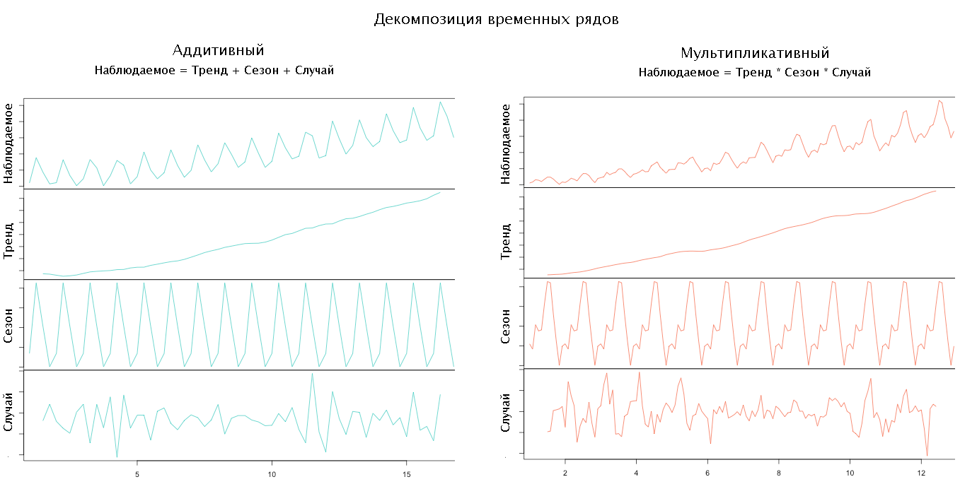
Source Anomaly.io
First, select the trend, smoothing the original data. The method and degree of smoothing are chosen by the researcher.
To determine the seasonal component from the source series, we subtract the trend or divide it into it, depending on the type of model chosen, and smooth it again. Then we divide the data by season (period), usually it is a week, and we find the average season. If the length of the season is not known, then you can try to find it:
For more information about models and decomposition, see the articles “Extract Seasonal & Trend: using decomposition in R” and “How To Identify Patterns in Time Series Data” .
Removing the trend and seasonal factor from the source series, we get a random component.
If we analyze only the random component, then many anomalies can be reduced to one of the following cases:
Of course, many algorithms for finding anomalies have already been implemented in the R language, intended for statistical data processing, in the form of packages: tsoutliers , strucchange , Twitter Anomaly Detection, and others . Read more about R in articles. And you already apply R in business? and My experience of introducing R. It would seem, connect packages and use. However, there is a problem - setting the parameters of statistical checks, which, unlike critical values, are far from obvious to most and do not have universal values. The way out of this situation can be a selection of brute force (resource-intensive), with a rare periodic refinement, independently for each metric. On the other hand, most non-seasonal anomalies are well defined visually, which suggests the use of a neural network on rendered graphs.
Below, I provide my own algorithms that work comparable to Twitter Breakout in terms of results, and somewhat faster in speed when implemented in Java Script.
Disclaimer
The author, although he has a mathematical education, is in no way connected with either Data Mining or statistical analysis. This material is the result of a study conducted to determine the possibility of writing an anomaly search module (even if it is weak) for the monitoring system being developed.
What are we looking for in two pictures
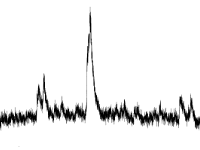
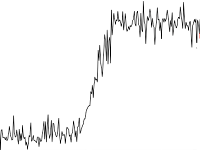
Examples of anomalies on the charts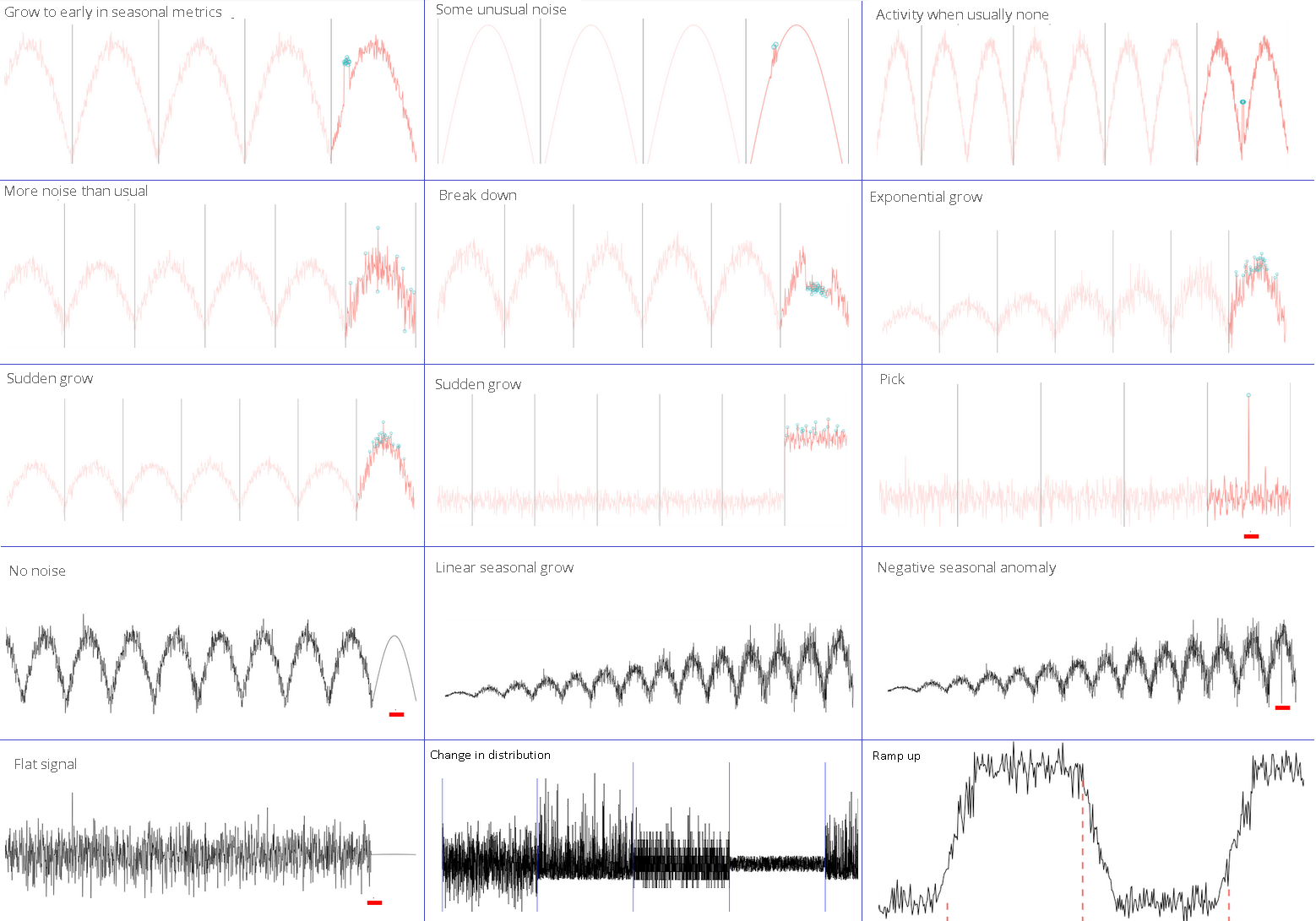
Source Anomaly.io
Of course, in reality, things are not always so simple: only on b), d) and e) an obvious anomaly.
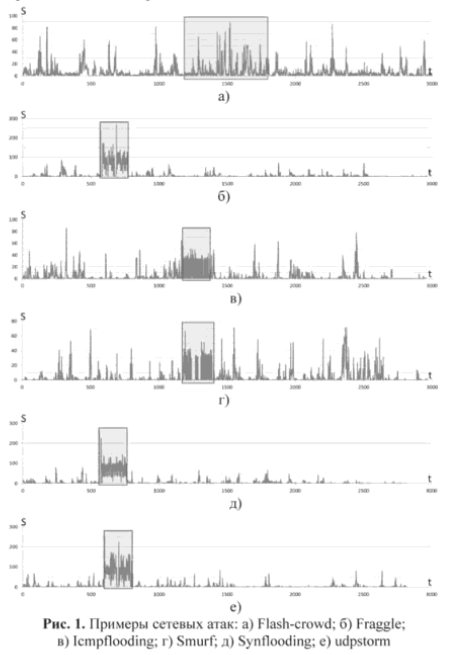
Source cyberleninka.ru
Source Anomaly.io
Of course, in reality, things are not always so simple: only on b), d) and e) an obvious anomaly.
Source cyberleninka.ru
Current state of affairs
Commercial products are almost always presented as a service, using both statistics and machine learning. Here are some of them: AIMS , Anomaly.io (an excellent blog with examples), CoScale (integration capabilities, for example with Zabbix), DataDog , Grok , Metricly.com and Azure (from Microsoft). Elastic has a machine-based X-Pack module.
')
Open-source products that can be deployed in:
- Atlas from Netflix - in-memory database for analyzing time series. The search is performed by Holt-Winters.
- Banshee by Eleme. Only one algorithm based on the three sigma rule is used for detection.
- Etsy's KALE stack, which consists of two Skyline products, for detecting problems in real time, and Oculus for finding relationships. Looks like abandoned.
- Morgoth is an anomaly detection framework in Kapacitor (InfluxDB notification module). Out of the box is: the three sigma rule, the Kolmogorov-Smirnov test and the Jensen-Shannon deviation .
- Prometheus is a popular monitoring system in which you can independently implement some search algorithms using standard functionality.
- RRDTool is a database used, for example, in Cacti and Munin. Able to make a forecast method Holt-Winters. How this can be used - in the article Monitoring Prediction, Potential Failure Alerts
- ~ 2000 repositories on github
In my opinion, open-source search quality is significantly inferior. To understand how the search for anomalies works and whether it is possible to correct the situation, it is necessary to plunge into statistics a little. Mathematical details are simplified and hidden under the spoilers.
Model and its components
For the analysis of the time series using a model that reflects the expected features (components) of the series. Usually a model consists of three components:
- Trend - reflects the overall behavior of the series in terms of increasing or decreasing values.
- Seasonality - periodic fluctuations of values associated, for example, with the day of the week or month.
- The random meaning is what will remain of the series after the exclusion of other components. Here we will look for anomalies.
You can include additional components, such as cyclical , as a trend multiplier,
abnormal (Catastrophic event) or social (holidays) . If the trend or seasonality in the data is not visible, then the corresponding components from the model can be excluded.
Depending on how the components of the model are interconnected, determine its type. So, if all components add up to get an observable series, then they say that the model is addictive, if they multiply, then they are multiplicative, if something multiplies, and something disappears, then mixed. Typically, the type of model is chosen by the researcher based on a preliminary analysis of the data.
Decomposition
By choosing the type of model and the set of components, you can proceed to decompose the time series, i.e. its decomposition into components.
Source Anomaly.io
First, select the trend, smoothing the original data. The method and degree of smoothing are chosen by the researcher.
Row smoothing methods: moving average, exponential smoothing and regression
The easiest way to smooth the time series is to use half the amount of the neighboring ones instead of the original values.
If you use not one, but several preceding values, i.e. arithmetic average of k-adjacent values, then such smoothing is called simple moving average with a window width k
If for each previous value to use some kind of a coefficient that determines the degree of influence on the current one, then we obtain a weighted moving average .
A slightly different way is to use exponential smoothing. The smoothed series is calculated as follows: the first element coincides with the first element of the original series, while the subsequent ones are calculated by the forum
Where α is the smoothing coefficient, from 0 to 1. As it is easy to see the closer α is to 1, the more the resulting series will be similar to the original.
To determine the linear trend, you can take the method of calculating the linear regression yt=a+bxt+ varepsilont least squares method : hatb= frac overlinexy overlinex2 , hata= bary−b barx where barx and bary - arithmetic average x and y .
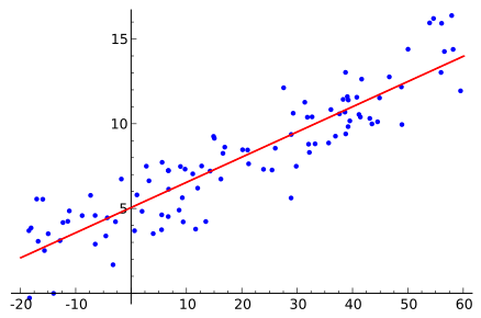
Source Wikipedia
sn= fracxn+xn−12
If you use not one, but several preceding values, i.e. arithmetic average of k-adjacent values, then such smoothing is called simple moving average with a window width k
sn= fracxn+xn−1+...+xn−kk
If for each previous value to use some kind of a coefficient that determines the degree of influence on the current one, then we obtain a weighted moving average .
A slightly different way is to use exponential smoothing. The smoothed series is calculated as follows: the first element coincides with the first element of the original series, while the subsequent ones are calculated by the forum
sn= alphaxn+(1− alpha)sn−1
Where α is the smoothing coefficient, from 0 to 1. As it is easy to see the closer α is to 1, the more the resulting series will be similar to the original.
To determine the linear trend, you can take the method of calculating the linear regression yt=a+bxt+ varepsilont least squares method : hatb= frac overlinexy overlinex2 , hata= bary−b barx where barx and bary - arithmetic average x and y .
Source Wikipedia
To determine the seasonal component from the source series, we subtract the trend or divide it into it, depending on the type of model chosen, and smooth it again. Then we divide the data by season (period), usually it is a week, and we find the average season. If the length of the season is not known, then you can try to find it:
Discrete Fourier Transform or Auto-Correlation
Honestly, I did not understand how the Fourier transform works. Who would be interested in looking at the following articles: Detect Seasonality using Fourier Transform in R and Simple words about the Fourier transform . As I understand it, the original series / function is represented as an infinite sum of elements and the first few significant coefficients are taken.
To search for auto-correlation, simply shift the function to the right and look for a position so that the distance / area between the original and the shifted function (highlighted in red) is minimal. Obviously, for the algorithm, the shift step and the maximum limit should be specified, when reached, we consider that the period search failed.
To search for auto-correlation, simply shift the function to the right and look for a position so that the distance / area between the original and the shifted function (highlighted in red) is minimal. Obviously, for the algorithm, the shift step and the maximum limit should be specified, when reached, we consider that the period search failed.
For more information about models and decomposition, see the articles “Extract Seasonal & Trend: using decomposition in R” and “How To Identify Patterns in Time Series Data” .
Removing the trend and seasonal factor from the source series, we get a random component.
Types of anomalies
If we analyze only the random component, then many anomalies can be reduced to one of the following cases:
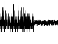
- Overshoot
 Finding outliers in the data is a classic problem for which there is already a good set of solutions:Three Sigma Rule, Interquartile Range and OthersThe idea of such tests is to determine how far an individual value from the average is located. If the distance is different from “normal”, the value is announced as an outlier. The time of the event is ignored.
We assume that the input is a series of numbers - x1 , x2 ... xn , Total n pieces xi - i th number.
Standard tests are fairly simple to implement and only require an average calculation. barx=(x1+...+xn)/n standard deviation S= sqrt frac1n−1 sumni=1 left(xi− barx right)2 and sometimes medians M - the average value, if you order all the numbers in ascending order and take the one that is in the middle.
Three Sigma Rule
If a |xi− barx|>3∗S then xi we consider as emission.
Z-score and updated method Iglewicz and Hoaglin
xi - emission, if |xi− barx|/S more than a predetermined threshold, usually equal to 3. In essence, the rewritten three sigma rule.
The refined method is as follows: for each number of the series we calculate |xi−M| and for the resulting values we find the median, denoted by MAD .
xi - emission, if 0.6745∗|xi−M|/MAD more than the threshold.
Interquartile range
We sort the initial numbers in ascending order, divide by two, and for each part we find the median values Q1 and Q3 .
xi - emission, if |xi−M|>1.5∗(Q3−Q1) .
Grubbs test
Find the minimum xmin and maximum xmax values and for them we calculate Gmin=( barx−xmin)/S and Gmax=(xmax− barx)/S . Then we choose the level of significance α (usually one of 0.01, 0.05 or 0.1), look in the table of critical values , choose a value for n and α. If a Gmin or Gmax more than the table value, then we consider the corresponding element of the series as an outlier
Tests usually require a normal distribution to be investigated, but often this requirement is ignored. - Shift
 The problem of detecting a shift in the data is well investigated, since it occurs in signal processing. To solve it, you can use Twitter Breakout Detection . I note that it works much worse if the initial series is analyzed with components of seasonality and trend.
 - Change in character (distribution) of values
 As for the shift, you can use the same BreakoutDetection package from Twitter, but not everything goes smoothly with it.
 - Deviation from “everyday” (for data with seasonality)
To detect this anomaly, it is necessary to compare the current period and several previous ones. Usually usedHolt Winters MethodThe method refers to the prediction, so its use is to compare the predicted value with the actual value.
The main idea of the method is that each of the three components is exponentially smoothed using a separate smoothing factor, so the method is often called triple exponential smoothing. The formulas for calculating the multiplicative and addictive seasons are in Wikipedia , and the details of the method in the article on Habré .
Three smoothing parameters should be chosen so that the resulting series was “close” to the original. In practice, this problem is solved by enumeration, although RRDTool requires explicit specification of these values.
Disadvantage of the method: requires at least three seasons of data.
Another method used in Odnoklassniki is to select values from other seasons that correspond to the analyzed moment, and check their totality for the presence of an outlier, for example, with the Grubbs test.
Twitter also offers AnomalyDetection , which on the test data shows good results. Unfortunately, like BreakoutDetection, it has been two years without updates. - Behavioral
Sometimes anomalies can be specific in nature, which in most cases should be ignored, for example, one value for two adjacent elements. In such cases, separate algorithms are required. - Joint anomalies
Separately, it is worth mentioning anomalies, when the values of two observable metrics of a series are within the normal range, but their joint appearance is a sign of a problem. In general, finding such anomalies can be solved by cluster analysis , when pairs of values represent the coordinates of points on the plane and the whole set of events is divided into two / three groups (clusters) - “norm” / “noise” and “anomaly”.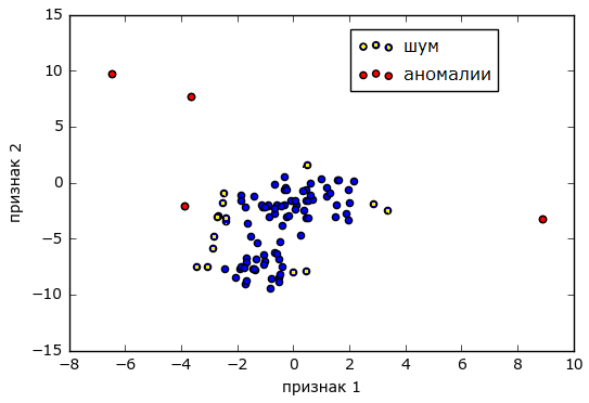
Source alexanderdyakonov.wordpress.com
A weaker method is to track how much the metrics depend on each other in time and in the case when the dependence is lost, to report an anomaly. For this, you can probably use one of the methods.Pearson linear correlation coefficientLet be x1,x2,...,xn and y1,y2,...,yn two sets of numbers and you want to find out if there is a linear relationship between them. Calculate for x the average barx=(x1+...+xn)/n and standard deviation Sx= sqrt frac1n−1 sumni=1 left(xi− barx right)2 . Similarly for y .
Pearson Correlation Coefficientr(x,y)= frac sumni=1(xi− barx)(yi− bary)SxSy
The closer the modulus is to 1, the greater the dependency. If the coefficient is closer to -1, then the dependence is inverse, i.e. growth x associated with decreasing y .Distance Damerau - LevenshteynSuppose there are two lines ABC and ADEC. To get the second out of the first one, you need to remove B and add D and E. If each of the operations of deleting / adding a character and permuting XY into YX specify a cost, then the total cost will be the distance Damerau – Levenshten.
To determine the similarity of the graphs, you can push off from the algorithm used in KALEInitially, the initial series of values, for example, a series of the form [960, 350, 350, 432, 390, 76, 105, 715, 715], is normalized: a maximum is searched for - it will correspond to 25, and a minimum - it will correspond to 0; thus, the data is proportionally distributed in the limit of integers from 0 to 25. As a result, we obtain a series of the form [25, 8, 8, 10, 9, 0, 1, 18, 18]. Then the normalized series is encoded using 5 words: sdec (sharply down), dec (down), s (exactly), inc (up), sinc (sharply up). The result is a series of the form [sdec, flat, inc, dec, sdec, inc, sinc, flat].
By coding two time series in this way, you can find out the distance between them. And if it is less than a certain threshold, then assume that the graphics are similar and there is a connection.
Conclusion
Of course, many algorithms for finding anomalies have already been implemented in the R language, intended for statistical data processing, in the form of packages: tsoutliers , strucchange , Twitter Anomaly Detection, and others . Read more about R in articles. And you already apply R in business? and My experience of introducing R. It would seem, connect packages and use. However, there is a problem - setting the parameters of statistical checks, which, unlike critical values, are far from obvious to most and do not have universal values. The way out of this situation can be a selection of brute force (resource-intensive), with a rare periodic refinement, independently for each metric. On the other hand, most non-seasonal anomalies are well defined visually, which suggests the use of a neural network on rendered graphs.
application
Below, I provide my own algorithms that work comparable to Twitter Breakout in terms of results, and somewhat faster in speed when implemented in Java Script.
Algorithm piecewise linear approximation of the time series
- If the row is very noisy, then we average, for example. on 5 elements.
- The result includes the first and last points of the series.
- Find the most distant point of the row from the current polyline and add it to the set.
- Repeat until the average deviation from the broken line to the original row is less than the average deviation in the original row or until the limit number of vertices of the broken line is reached (in this case, the approximation probably did not succeed).
Algorithm for finding the shift in the data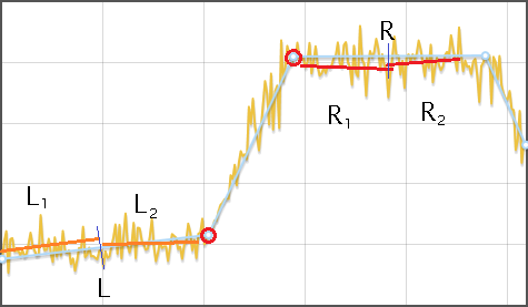
- Approximate the original row of broken line
- For each line segment, except the first and last:
- Find its height h , as the difference of y-coordinates of the beginning and end. If the height is less than the ignored interval, then this segment is ignored.
- Both adjacent segments L and R divide by two, each plot L1 , L2 , R1 , R2 approximate by its straight line and find the average distance from the straight line to the row - dL1 , dL2 , dR1 , dR2 .
- If a |dL1−dL2| and |dR1−dR2| significantly less than h then consider that a shift is detected
Algorithm for Finding Changes in Distribution
- The original series is divided into segments, long, depending on the number of data, but not less than three.
- Each segment is searched for a minimum and maximum. Replacing each segment with its center, two rows are formed - minima and maxima. Further rows are processed separately.
- The series is linearly approximated and for each of its vertices, except the first and last, a comparison of the data of the original series, lying to the right and to the adjacent vertices of the polyline, is carried out by the Kolmogorov-Smirnov test. If a difference is found, the point is added to the result.
Kolmogorov-Smirnov test
Let be x1,x2,...,xn1 and y1,y2,...,yn2 two sets of numbers and is required to assess the materiality of the differences between them.
Initially, the values of both rows are divided into several (about a dozen) categories. Next for each category is calculated the number fx the values from the series x and divided by row length n1 . Similarly for a number y . For each category we find |fx−fy| and then the total maximum dmax in all categories. The test value of the criterion is calculated by the formula lambda=dmax fracn1n2n1+n2 .
The level of significance is selected. alpha (one of 0.01, 0.05, 0.1) and by it is determined by the critical value of the table . If a lambda more critical values, it is believed that the groups differ significantly.
Source: https://habr.com/ru/post/344762/
All Articles